The routine may be called by the names d01esf or nagf_quad_md_sgq_multi_vec.
3Description
d01esf uses a sparse grid to generate a vector of approximations to a vector of integrals over the unit hypercube , that is,
3.1Comparing Quadrature Over Full and Sparse Grids
Before illustrating the sparse grid construction, it is worth comparing integration over a sparse grid to integration over a full grid.
Given a one-dimensional quadrature rule with abscissae, which accurately evaluates a polynomial of order , a full tensor product over dimensions, a full grid, may be constructed with multidimensional abscissae. Such a product will accurately integrate a polynomial where the maximum power of any dimension is . For example if and , such a rule will accurately integrate any polynomial whose highest order term is . Such a polynomial may be said to have a maximum combined order of , provided no individual dimension contributes a power greater than . However, the number of multidimensional abscissae, or points, required increases exponentially with the dimension, rapidly making such a construction unusable.
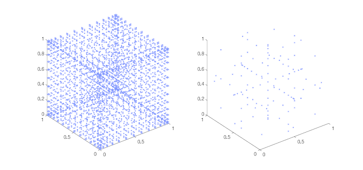
The sparse grid technique was developed by Smolyak (Smolyak (1963)). In this, multiple one-dimensional quadrature rules of increasing accuracy are combined in such a way as to provide a multidimensional quadrature rule which will accurately evaluate the integral of a polynomial whose maximum order appears as a monomial. Hence a sparse grid construction whose highest level quadrature rule has polynomial order will accurately integrate a polynomial whose maximum combined order is also . Again taking , one may, theoretically, accurately integrate a polynomial such as , but not a polynomial such as . Whilst this has a lower maximum combined order than the full tensor product, the number of abscissae required increases significantly slower than the equivalent full grid, making some classes of integrals of dimension tractable. Specifically, if a one-dimensional quadrature rule of level has abscissae, the corresponding full grid will have multidimensional abscissae, whereas the sparse grid will have . Figure 1 demonstrates this using a Gauss–Patterson rule with points in dimensions. The full grid requires points, whereas the sparse grid only requires .
Figure 1: Three-dimensional full (left) and sparse (right) grids, constructed from the point Gauss–Patterson rule
3.2Sparse Grid Quadrature
We now include a brief description of the sparse grid construction, sufficient for the understanding of the use of this routine. For a more detailed analysis, see Gerstner and Griebel (1998).
Consider a one-dimensional -point quadrature rule of level , . The action of this rule on a integrand is to approximate its definite one-dimensional integral as,
using weights and abscissae , for .
Now construct a set of one-dimensional quadrature rules, , such that the accuracy of the quadrature rule increases with the level number. In this routine we exclusively use quadrature rules which are completely nested, implying that if an abscissae is in level , it is also in level . The quantity denotes some maximum level appropriate to the rules that have been selected.
Now define the action of the tensor product of rules as,
where the individual level indices are not necessarily ordered or unique. Each tensor product of rules defines an action of the quadrature rules , over a subspace, which is given a level . If all rule levels are equal, this is the full tensor product of that level.
The sparse grid construction of level can then be declared as the sum of all actions of the quadrature differences , over all subspaces having a level at most ,
(1)
By definition, all subspaces used for level must also be used for level , and as such the difference between the result of all actions over subsequent sparse grid constructions may be used as an error estimate.
Let be the maximum level allowable in a sparse grid construction. The classical sparse grid construction of allows each dimension to support a one-dimensional quadrature rule of level at most , with such a quadrature rule being used in every dimension at least once. Such a construction lends equal weight to each dimension of the integration, and is termed here ‘isotropic’.
Define the set , where is the maximum quadrature rule allowed in the th dimension, and to be the maximum quadrature rule used by any dimension. Let a subspace be identified by its quadrature difference levels, .
The classical construction may be extended by allowing different dimensions to have different values , and by allowing . This creates non-isotropic constructions. These are especially useful in higher dimensions, where some dimensions contribute more than others to the result, as they can drastically reduce the number of function evaluations required.
For example, consider the two-dimensional construction with . The classical isotropic construction would have the following subspaces.
Subspaces generated by a classical sparse grid with .
Level
Subspaces
,
,
,
,
,
,
If the variation in the second dimension is sufficiently accurately described by a quadrature rule of level , the contributions of the subspaces and are probably negligible. Similarly, if the variation in the first dimension is sufficiently accurately described by a quadrature rule of level , the subspace is probably negligible. Furthermore the subspace would also probably have negligible impact, whereas the subspaces and would not. Hence restricting the first dimension to a maximum level of , and the second dimension to a maximum level of would probably give a sufficiently acceptable estimate, and would generate the following subspaces.
Subspaces generated by a non-isotropic sparse grid with , and .
Level
Subspaces
,
,
,
Taking this to the extreme, if the variation in the first and second dimensions are sufficiently accurately described by a level quadrature rule, restricting the maximum level of both dimensions to would generate the following subspaces.
Subspaces generated by a sparse grid construction with , and .
Level
Subspaces
,
None
Hence one subspace is generated at level , and no subspaces are generated at level . The level subspace actually indicates that this is the full grid of level .
3.3Using d01esf
d01esf uses optional parameters, supplied in the option arrays iopts and opts. Before calling d01esf, these option arrays must be initialized using d01zkf. Once initialized, the required options may be set and queried using d01zkf and d01zlf respectively. A complete list of the options available may be found in Section 11.
You may control the maximum level required, , using the optional parameter Maximum Level. Furthermore, you may control the first level at which the error comparison will take place using the optional parameter Minimum Level, allowing for the forced evaluation of a predetermined number of levels before the routine attempts to complete. Completion is flagged when the error estimate is sufficiently small:
where and are the absolute and relative error tolerances, respectively, and is the highest level at which computation was performed. The tolerances and can be controlled by setting the optional parameters Absolute Tolerance and Relative Tolerance.
Owing to the interlacing nature of the quadrature rules used herein, abscissae required in lower level subspaces will also appear in higher-level subspaces. This allows for calculations which will be repeated later to be stored and re-used. However, this is naturally at the expense of memory. It may also be at the expense of computational time, depending on the complexity of the integrands, as the lookup time for a given value is (at worst) . Furthermore, as the sparse grid level increases, fewer subsequent levels will require values from the current level. You may control the number of levels for which values are stored by setting the optional parameter Index Level.
Two different sets of interlacing quadrature rules are selectable using the optional parameter Quadrature Rule: Gauss–Patterson and Clenshaw–Curtis. Gauss–Patterson rules offer greater polynomial accuracy, whereas Clenshaw–Curtis rules are often effective for oscillatory integrands. Clenshaw–Curtis rules require function values to be evaluated on the boundary of the hypercube, whereas Gauss–Patterson rules do not. Both of these rules use precomputed weights, and as such there is an effective limit on ; see the description of the optional parameter Quadrature Rule. The value of is returned by the queriable optional parameter Maximum Quadrature Level.
d01esf also allows for non-isotropic sparse grids to be constructed. This is done by appropriately setting the array maxdlv. It should be emphasised that a non-isometric construction should only be used if the integrands behave in a suitable way. For example, they may decay toward zero as the lesser dimensions approach their bounds of . It should also be noted that setting will not reduce the dimension of the integrals, it will simply indicate that only one point in dimension should be used. It is also advisable to approximate the integrals several times, once with an isometric construction of some level, and then with a non-isometric construction with higher levels in various dimensions. If the difference between the solutions is significantly more than the returned error estimates, the assumptions of dimensional importance are probably incorrect.
The abscissae in each subspace are generally expressible in a sparse manner, because many of the elements of each abscissa will in fact be the centre point of the dimension, which is termed here the ‘trivial’ element. In this routine the trivial element is always returned as owing to the restriction to the hypercube. As such, the subroutine f returns the abscissae in Compressed Column Storage (CCS) format (see the F11 Chapter Introduction). This has particular advantages when using accelerator hardware to evaluate the required functions, as much less data must be forwarded. It also, potentially, allows for calculations to be computed faster, as any sub-calculations dependent upon the trivial value may be potentially re-used.
4References
Caflisch R E, Morokoff W and Owen A B (1997) Valuation of mortgage backed securities using Brownian bridges to reduce effective dimension Journal of Computational Finance1 27–46
Gerstner T and Griebel M (1998) Numerical integration using sparse grids Numerical Algorithms18 209–232
Smolyak S A (1963) Quadrature and interpolation formulas for tensor products of certain classes of functions Dokl. Akad. Nauk SSSR4 240–243
5Arguments
1: – IntegerInput
On entry: , the number of integrands.
Constraint:
.
2: – IntegerInput
On entry: , the number of dimensions.
Constraint:
.
3: – Subroutine, supplied by the user.External Procedure
f must return the value of the integrands at a set of -dimensional points , implicitly supplied as columns of a matrix . If was supplied explicitly you would find that most of the elements attain the same value, ; the larger the number of dimensions, the greater the proportion of elements of would be equal to . So, is effectively a sparse matrix, except that the ‘zero’ elements are replaced by elements that are all equal to the value . For this reason is supplied, as though it were a sparse matrix, in compressed column storage (CCS) format (see the F11 Chapter Introduction).
Individual entries
of , for , are either trivially valued, in which case , or are non-trivially valued. For point , the non-trivial row indices and corresponding abscissae values are supplied in elements
, for , of the arrays irowix and xs, respectively. Hence the th column of the matrix is retrievable as
An equivalent integer valued matrix is also implicitly provided. This contains the unique indices of the underlying one-dimensional quadrature rule corresponding to the individual abscissae . For trivial abscissae, the implicit index . is supplied in the same CCS format as , with the non-trivial values supplied in qs.
On entry: , the number of points , corresponding to the number of columns of , at which the set of integrands must be evaluated.
4: – Real (Kind=nag_wp)Input
On entry: , the value of the trivial elements of .
5: – IntegerInput
On entry: if , the number of non-trivial elements of .
If , the total number of abscissae from the underlying one-dimensional quadrature.
6: – Integer arrayInput
On entry: the set contains the indices of irowix and xs corresponding to the non-trivial elements of column of and hence of the point , for .
7: – Integer arrayInput
On entry: the row indices corresponding to the non-trivial elements of .
8: – Real (Kind=nag_wp) arrayInput
On entry: , the non-trivial entries of .
9: – Integer arrayInput
On entry: , the indices of the underlying quadrature rules corresponding to .
10: – Real (Kind=nag_wp) arrayOutput
On exit: , for and .
11: – IntegerInput/Output
On entry: if , this is the first call to f. , and the entire point will satisfy , for . In addition, nntr contains the total number of abscissae from the underlying one-dimensional quadrature; xs contains the complete set of abscissae and qs contains the corresponding quadrature indices, with and . This will always be called in serial.
In subsequent calls to f, . Subsequent calls may be made from within an OpenMP parallel region. See Section 8 for details.
On exit: set if you wish to force an immediate exit from d01esf with .
12: – Integer arrayUser Workspace
13: – Real (Kind=nag_wp) arrayUser Workspace
f is called with the arguments iuser and ruser as supplied to d01esf. You should use the arrays iuser and ruser to supply information to f.
f must either be a module subprogram USEd by, or declared as EXTERNAL in, the (sub)program from which d01esf is called. Arguments denoted as Input must not be changed by this procedure.
Note:f should not return floating-point NaN (Not a Number) or infinity values, since these are not handled by d01esf. If your code inadvertently does return any NaNs or infinities, d01esf is likely to produce unexpected results.
4: – Integer arrayInput
On entry: , the array of maximum levels for each dimension.
, for , contains , the maximum level of quadrature rule dimension j will support.
If for all , only one evaluation will be performed, and as such no error estimation will be possible.
Suggested value:
for all .
Note: setting non-default values for some dimensions makes the assumption that the contribution from the omitted subspaces is . The integral and error estimates will only be based on included subspaces, which if the contribution assumption is not valid will be erroneous.
5: – Real (Kind=nag_wp) arrayOutput
On exit: contains the final estimate of the definite integral , for .
6: – Real (Kind=nag_wp) arrayOutput
On exit: contains the final error estimate of the definite integral , for .
7: – Integer arrayOutput
On exit: indicates the final state of integral , for .
The error estimate for integral was below the requested tolerance.
The error estimate for integral was below the requested tolerance. The final level used was non-isotropic.
The error estimate for integral was above the requested tolerance.
The error estimate for integral was above .
You aborted the evaluation before an error estimate could be made.
8: – Integer arrayCommunication Array
9: – Real (Kind=nag_wp) arrayCommunication Array
The arrays iopts and optsmust not be altered between calls to any of the routines d01esf,d01zkfandd01zlf.
10: – Integer arrayUser Workspace
11: – Real (Kind=nag_wp) arrayUser Workspace
iuser and ruser are not used by d01esf, but are passed directly to f and may be used to pass information to this routine.
12: – IntegerInput/Output
On entry: ifail must be set to , or to set behaviour on detection of an error; these values have no effect when no error is detected.
A value of causes the printing of an error message and program execution will be halted; otherwise program execution continues. A value of means that an error message is printed while a value of means that it is not.
If halting is not appropriate, the value or is recommended. If message printing is undesirable, then the value is recommended. Otherwise, the value is recommended since useful values can be provided in some output arguments even when on exit. When the value or is used it is essential to test the value of ifail on exit.
On exit: unless the routine detects an error or a warning has been flagged (see Section 6).
6Error Indicators and Warnings
If on entry or , explanatory error messages are output on the current error message unit (as defined by x04aaf).
Errors or warnings detected by the routine:
Note: in some cases d01esf may return useful information.
The requested accuracy was not achieved for at least one integral.
No accuracy was achieved for at least one integral.
On entry, . Constraint: .
On entry, . Constraint: .
Either the option arrays iopts and opts have not been initialized for d01esf, or they have become corrupted.
An unexpected error has been triggered by this routine. Please
contact NAG.
See Section 7 in the Introduction to the NAG Library FL Interface for further information.
Your licence key may have expired or may not have been installed correctly.
See Section 8 in the Introduction to the NAG Library FL Interface for further information.
Dynamic memory allocation failed.
See Section 9 in the Introduction to the NAG Library FL Interface for further information.
7Accuracy
For each integral , an error estimate is returned, where,
where is the highest level at which computation was performed.
8Parallelism and Performance
8.1Direct Threading
d01esf is directly threaded for parallel execution. For each level, at most threads will evaluate the integrands over independent subspaces of the construction, and will construct a partial sum of the level's contribution. Once all subspaces from a given level have been processed, the partial sums are combined to give the total contribution of the level, which is in turn added to the total solution. For a given number of threads, the division of subspaces between the threads, and the order in which a single thread operates over its assigned subspaces, is fixed. However, the order in which all subspaces are combined will necessarily be different to the single threaded case, which may result in some discrepency in the results between parallel and serial execution.
To mitigate this discrepency, it is recommended that d01esf be instructed to use higher-than-working precision to accumulate the actions over the subspaces. This is done by setting the option , which is the default behaviour. This has some computational cost, although this is typically negligible in comparison to the overall runtime, particularly for non-trivial integrands.
If , then the accumulation will be performed using working precision, which may provide some increase in performance. Again, this is probably negligible in comparison to the overall runtime.
For some problems, typically of lower dimension, there may be insufficient work to warrant direct threading at lower levels. For example, a three-dimensional problem will require at most subspaces to be evaluated at level , and at most subspaces at level . Furthermore, level subspaces typically contain only new multidimensional abscissae, while level subspaces typically contain or new multidimensional abscissae depending on the Quadrature Rule. If there are more threads than the number of available subspaces at a given level, or the amount of work in each subspace is outweighed by the amount of work required to generate the parallel region, parallel efficiency will be decreased. This may be mitigated to some extent by evaluating the first levels in serial. The value of may be altered using the optional parameter Serial Levels. If , then all levels will be evaluated in serial and no direct threading will be utilized.
If you use direct threading in the manner just described, you must ensure any access to the
user arrays
iuser and ruser is done in a thread safe manner.
These are
classed as OpenMP SHARED, and
are
passed directly to the subroutine f for every thread.
The vectorized interface also allows for parallelization inside the subroutine f by evaluating the required integrands in parallel. Provided the values returned by f match those that would be returned without parallelizing f, the final result should match the serial result, barring any discrepencies in accumulation. If you wish to parallelize f, it is advisable to set a large value for Maximum Nx, although be aware that increasing Maximum Nx will increase the memory requirement of the routine. In general, parallelization of f should not be necessary, as the higher-level parallelism over different subspaces scales well for many problems.
9Further Comments
Not applicable.
10Example
The example program evaluates an estimate to the set of integrals
where .
It also demonstrates a simple method to safely use iuser and ruser as workspace for sub-calculations when running in parallel.
Several optional parameters in d01esf control aspects of the algorithm, methodology used, logic or output. Their values are contained in the arrays iopts and opts; these must be initialized before calling d01esf by first calling d01zkf with optstr set to "Initialize = d01esf".
Each optional parameter has an associated default value; to set any of them to a non-default value, or to reset any of them to the default value, use d01zkf. The current value of an optional parameter can be queried using d01zlf.
The remainder of this section can be skipped if you wish to use the default values for all optional parameters.
The following is a list of the optional parameters available. A full description of each optional parameter is provided in Section 11.1.
All options accept the value ‘DEFAULT’ in order to return single options to their default states.
Keywords and character values are case insensitive, however they must be separated by at least one space.
Queriable options will return the appropriate value when queried by calling d01zlf. They will have no effect if passed to d01zkf.
For d01esf the maximum length of the argument cvalue used by d01zlf is .
Absolute Tolerance
Default
, the absolute tolerance required.
Index Level
Default
The maximum level at which function values are stored for later use. Larger values use increasingly more memory, and require more time to access specific elements. Lower levels result in more repeated computation. The Maximum Quadrature Level, is the effective upper limit on Index Level. If , d01esf will use as the value of Index Level.
Constraint: .
Maximum Level
Default
, the maximum number of levels to evaluate.
Constraint: .
Note: the maximum allowable level in any single dimension, , is governed by the Quadrature Rule selected. If a value greater than is set, only a subset of subspaces from higher levels will be used. Should this subset be empty for a given level, computation will consider the preceding level to be the maximum level and will terminate.
Maximum Nx
Default
, the maximum number of points to evaluate in a single call to f.
Constraint: .
Maximum Quadrature Level
Queriable only
, the maximum level of the underlying one-dimensional quadrature rule (see Quadrature Rule).
Minimum Level
Default
The minimum number of levels which must be evaluated before an error estimate is used to determine convergence.
Constraint: .
Note: if the minimum level is greater than the maximum computable level, the maximum level will be used.
Quadrature Rule
Default
The underlying one-dimensional quadrature rule to be used in the construction. Open rules do not require evaluations at boundaries.
or
The interlacing Gauss–Patterson rules. Level uses abscissae. All levels are open. These rules provide high order accuracy. .
or
The interlacing Clenshaw–Curtis rules. Level uses abscissae. All levels above level are closed. .
Relative Tolerance
Default
, the relative tolerance required.
Summation Precision
Default
Determines whether d01esf uses working precision or higher-than-working precision to accumulate the actions over subspaces.
or
Higher-than-working precision is used to accumulate the action over a subspace, and for the accumulation of all such actions. This is more expensive computationally, although this is probably negligible in comparison to the cost of evaluating the integrands and the overall runtime. This significantly reduces variation in the result when changing the number of threads.
or
Working precision is used to accumulate the actions over subspaces. This may provide some speedup, particularly if or is large. The results of parallel simulations will however be more prone to variation.
Note: the following option is relevant only to multithreaded implementations of the NAG Library.
Serial Levels
Default
, the number of levels to be evaluated in serial before initializing parallelization. For relatively trivial integrands, this may need to be set greater than the default to reduce parallel overhead.