This chapter provides functions for the solution of systems of simultaneous linear equations, and associated computations. It provides functions for
matrix factorizations;
solution of linear equations;
estimating matrix condition numbers;
computing error bounds for the solution of linear equations;
matrix inversion.
Functions are provided for both real and complex data.
For a general introduction to the solution of systems of linear equations, you should turn first to the F04 Chapter Introduction. The decision trees, in Section 4 in the F04 Chapter Introduction, direct you to the most appropriate functions in Chapters F04 or F07 for solving your particular problem. In particular, Chapters F04 and F07 contain Black Box (or driver) functions which enable some standard types of problem to be solved by a call to a single function. Where possible, functions in Chapter F04 call Chapter F07 functions to perform the necessary computational tasks.
There are two types of driver functions in this chapter: simple drivers which just return the solution to the linear equations; and expert drivers which also return condition and error estimates and, in many cases, also allow equilibration. The simple drivers for real matrices have names of the form
nag_d..sv (f07.ac)
and for complex matrices have names of the form
nag_z..sv (f07.nc).
The expert drivers for real matrices have names of the form
nag_d..svx (f07.bc)
and for complex matrices have names of the form
nag_z..svx (f07.pc).
The functions in this chapter (Chapter F07) handle only dense and band matrices (not matrices with more specialised structures, or general sparse matrices).
The functions in this chapter have all been derived from the LAPACK project (see Anderson et al. (1999)). They have been designed to be efficient on a wide range of high-performance computers, without compromising efficiency on conventional serial machines.
2Background to the Problems
This section is only a brief introduction to the numerical solution of systems of linear equations. Consult a standard textbook, for example Golub and Van Loan (1996) for a more thorough discussion.
2.1Notation
We use the standard notation for a system of simultaneous linear equations:
(1)
where is the coefficient matrix, is the right-hand side, and is the solution. is assumed to be a square matrix of order .
If there are several right-hand sides, we write
(2)
where the columns of are the individual right-hand sides, and the columns of are the corresponding solutions.
We also use the following notation, both here and in the function documents:
a computed solution to , (which usually differs from the exact solution because of round-off error)
the residual corresponding to the computed solution
the -norm of the vector
the -norm of the vector
the -norm of the matrix
the -norm of the matrix
the vector with elements
the matrix with elements
Inequalities of the form are interpreted component-wise, that is for all .
2.2Matrix Factorizations
If is upper or lower triangular, can be solved by a straightforward process of backward or forward substitution.
Otherwise, the solution is obtained after first factorizing , as follows.
General matrices (LU factorization with partial pivoting)
where is a permutation matrix, is lower-triangular with diagonal elements equal to , and is upper-triangular; the permutation matrix (which represents row interchanges) is needed to ensure numerical stability.
where is a permutation matrix, is upper triangular and is lower triangular. The permutation matrix (which represents row-and-column interchanges) is needed to ensure numerical stability and to reveal the numerical rank of .
where is a permutation matrix, is upper triangular, is lower triangular, and is a block diagonal matrix with diagonal blocks of order or ; and have diagonal elements equal to , and have unit matrices on the diagonal corresponding to the blocks of . The permutation matrix (which represents symmetric row-and-column interchanges) and the blocks in are needed to ensure numerical stability. If is in fact positive definite, no interchanges are needed and the factorization reduces to or with diagonal , which is simply a variant form of the Cholesky factorization.
2.3Solution of Systems of Equations
Given one of the above matrix factorizations, it is straightforward to compute a solution to by solving two subproblems, as shown below, first for and then for . Each subproblem consists essentially of solving a triangular system of equations by forward or backward substitution; the permutation matrix and the block diagonal matrix introduce only a little extra complication:
Frequently, in practical problems the data and are not known exactly, and it is then important to understand how uncertainties or perturbations in the data can affect the solution.
If is the exact solution to , and is the exact solution to a perturbed problem , then
where is the condition number of defined by
(3)
In other words, relative errors in or may be amplified in by a factor . Section 2.4.2 discusses how to compute or estimate .
Similar considerations apply when we study the effects of rounding errors introduced by computation in finite precision. The effects of rounding errors can be shown to be equivalent to perturbations in the original data, such that and are usually at most , where is the machine precision and is an increasing function of which is seldom larger than (although in theory it can be as large as ).
In other words, the computed solution is the exact solution of a linear system which is close to the original system in a normwise sense.
2.4.2Estimating condition numbers
The previous section has emphasized the usefulness of the quantity in understanding the sensitivity of the solution of . To compute the value of from equation (3) is more expensive than solving in the first place. Hence it is standard practice to estimate , in either the -norm or the -norm, by a method which only requires additional operations, assuming that a suitable factorization of is available.
The method used in this chapter is Higham's modification of Hager's method (see Higham (1988)). It yields an estimate which is never larger than the true value, but which seldom falls short by more than a factor of (although artificial examples can be constructed where it is much smaller). This is acceptable since it is the order of magnitude of which is important rather than its precise value.
Because is infinite if is singular, the functions in this chapter actually return the reciprocal of .
2.4.3Scaling and Equilibration
The condition of a matrix and hence the accuracy of the computed solution, may be improved by scaling; thus if and are diagonal matrices with positive diagonal elements, then
is the scaled matrix. A general matrix is said to be equilibrated if it is scaled so that the lengths of its rows and columns have approximately equal magnitude. Similarly a general matrix is said to be row-equilibrated (column-equilibrated) if it is scaled so that the lengths of its rows (columns) have approximately equal magnitude. Note that row scaling can affect the choice of pivot when partial pivoting is used in the factorization of .
A symmetric or Hermitian positive definite matrix is said to be equilibrated if the diagonal elements are all approximately equal to unity.
Functions are provided to return the scaling factors that equilibrate a matrix for general, general band, symmetric and Hermitian positive definite and symmetric and Hermitian positive definite band matrices.
2.4.4Componentwise error bounds
A disadvantage of normwise error bounds is that they do not reflect any special structure in the data and – that is, a pattern of elements which are known to be zero – and the bounds are dominated by the largest elements in the data.
Componentwise error bounds overcome these limitations. Instead of the normwise relative error, we can bound the relative error in each component of and :
where the component-wise backward error bound is given by
Functions are provided in this chapter which compute , and also compute a forward error bound which is sometimes much sharper than the normwise bound given earlier:
Care is taken when computing this bound to allow for rounding errors in computing . The norm is estimated cheaply (without computing ) by a modification of the method used to estimate .
2.4.5Iterative refinement of the solution
If is an approximate computed solution to , and is the corresponding residual, then a procedure for iterative refinement of can be defined as follows, starting with :
for , until convergence
compute
solve
compute
In Chapter F04, functions are provided which perform this procedure using additional precision to compute , and are thus able to reduce the forward error to the level of machine precision.
The functions in this chapter do not use additional precision to compute , and cannot guarantee a small forward error, but can guarantee a small backward error (except in rare cases when is very ill-conditioned, or when and are sparse in such a way that has a zero or very small component). The iterations continue until the backward error has been reduced as much as possible; usually only one iteration is needed.
2.5Matrix Inversion
It is seldom necessary to compute an explicit inverse of a matrix. In particular, do not attempt to solve by first computing and then forming the matrix-vector product ; the procedure described in Section 2.3 is more efficient and more accurate.
However, functions are provided for the rare occasions when an inverse is needed, using one of the factorizations described in Section 2.2.
2.6Packed Storage Formats
Functions which handle symmetric matrices are usually designed so that they use either the upper or lower triangle of the matrix; it is not necessary to store the whole matrix. If the upper or lower triangle is stored conventionally in the upper or lower triangle of a two-dimensional array, the remaining elements of the array can be used to store other useful data.
However, that is not always convenient, and if it is important to economize on storage, the upper or lower triangle can be stored in a one-dimensional array of length or a two-dimensional array with elements; in other words, the storage is almost halved.
The one-dimensional array storage format is referred to as packed storage; it is described in Section 3.4.2. The two-dimensional array storage format is referred to as Rectangular Full Packed (RFP) format; it is described in Section 3.4.3. They may also be used for triangular matrices.
Functions designed for these packed storage formats perform the same number of arithmetic operations as functions which use conventional storage. Those using a packed one-dimensional array are usually less efficient, especially on high-performance computers, so there is then a trade-off between storage and efficiency. The RFP functions are as efficient as for conventional storage, although only a small subset of functions use this format.
2.7Band and Tridiagonal Matrices
A band matrix is one whose nonzero elements are confined to a relatively small number of subdiagonals or superdiagonals on either side of the main diagonal. A tridiagonal matrix is a special case of a band matrix with just one subdiagonal and one superdiagonal. Algorithms can take advantage of bandedness to reduce the amount of work and storage required. The storage scheme used for band matrices is described in Section 3.4.4.
The factorization for general matrices, and the Cholesky factorization for symmetric and Hermitian positive definite matrices both preserve bandedness. Hence functions are provided which take advantage of the band structure when solving systems of linear equations.
The Cholesky factorization preserves bandedness in a very precise sense: the factor or has the same number of superdiagonals or subdiagonals as the original matrix. In the factorization, the row-interchanges modify the band structure: if has subdiagonals and superdiagonals, then is not a band matrix but still has at most nonzero elements below the diagonal in each column; and has at most superdiagonals.
The Bunch–Kaufman factorization does not preserve bandedness, because of the need for symmetric row-and-column permutations; hence no functions are provided for symmetric indefinite band matrices.
The inverse of a band matrix does not in general have a band structure, so no functions are provided for computing inverses of band matrices.
2.8Block Partitioned Algorithms
Many of the functions in this chapter use what is termed a block partitioned algorithm. This means that at each major step of the algorithm a block of rows or columns is updated, and most of the computation is performed by matrix-matrix operations on these blocks. The matrix-matrix operations are performed by calls to the Level 3 BLAS
(see Chapter F16),
which are the key to achieving high performance on many modern computers. See Golub and Van Loan (1996) or Anderson et al. (1999) for more about block partitioned algorithms.
The performance of a block partitioned algorithm varies to some extent with the block size – that is, the number of rows or columns per block. This is a machine-dependent argument, which is set to a suitable value when the Library is implemented on each range of machines. You do not normally need to be aware of what value is being used. Different block sizes may be used for different functions. Values in the range to are typical.
On some machines there may be no advantage from using a block partitioned algorithm, and then the functions use an unblocked algorithm (effectively a block size of ), relying solely on calls to the Level 2 BLAS
(see Chapter F16
again).
2.9Mixed Precision LAPACK Routines
Some LAPACK routines use mixed precision arithmetic in an effort to solve problems more efficiently on modern hardware. They work by converting a double precision problem into an equivalent single precision problem, solving it and then using iterative refinement in double precision to find a full precision solution to the original problem. The method may fail if the problem is too ill-conditioned to allow the initial single precision solution, in which case the functions fall back to solve the original problem entirely in double precision. The vast majority of problems are not so ill-conditioned, and in those cases the technique can lead to significant gains in speed without loss of accuracy. This is particularly true on machines where double precision arithmetic is significantly slower than single precision.
3Recommendations on Choice and Use of Available Functions
3.1Available Functions
Tables 1 and 8 in Section 3.6 show the functions which are provided for performing different computations on different types of matrices. Table 1 shows functions for real matrices; Table 8 shows functions for complex matrices. Each entry in the table gives the NAG function name and the LAPACK double precision name (see Section 3.3).
Functions are provided for the following types of matrix:
general
general band
symmetric or Hermitian positive definite
symmetric or Hermitian positive definite (packed storage)
symmetric or Hermitian positive definite (RFP storage)
symmetric or Hermitian positive definite band
symmetric or Hermitian positive definite tridiagonal
symmetric or Hermitian indefinite
symmetric or Hermitian indefinite (packed storage)
triangular
triangular (packed storage)
triangular (RFP storage)
triangular band
For each of the above types of matrix (except where indicated), functions are provided to perform the following computations:
(a)(except for RFP matrices) solve a system of linear equations (driver functions);
(b)(except for RFP matrices) solve a system of linear equations with condition and error estimation (expert drivers);
(c)(except for triangular matrices) factorize the matrix (see Section 2.2);
(d)solve a system of linear equations, using the factorization (see Section 2.3);
(e)(except for RFP matrices) estimate the condition number of the matrix, using the factorization (see Section 2.4.2); these functions also require the norm of the original matrix (except when the matrix is triangular) which may be computed by a function in
Chapter F16;
(f)(except for RFP matrices) refine the solution and compute forward and backward error bounds (see Sections 2.4.4 and 2.4.5); these functions require the original matrix and right-hand side, as well as the factorization returned from (a) and the solution returned from (b);
(g)(except for band and tridiagonal matrices) invert the matrix, using the factorization (see Section 2.5).
Thus, to solve a particular problem, it is usually only necessary to call a single driver function, but alternatively two or more functions may be called in succession. This is illustrated in the example programs in the function documents.
3.2NAG Names and LAPACK Names
As well as the NAG function name (beginning f07), Tables 1 and 8 show the LAPACK routine names in double precision.
The functions may be called either by their NAG short names or by their NAG long names. The NAG long names for a function is simply the LAPACK name (in lower case) prepended by nag_, for example, nag_lapacklin_dpotrf is the long name for f07fdc.
References to Chapter F07 functions in the manual normally include the LAPACK double precision names, for example, f07adc.
The LAPACK routine names follow a simple scheme. Most names have the structure xyyzzz, where the components have the following meanings:
–the initial letter x indicates the data type (real or complex) and precision:
s
real, single precision
d
real, double precision
c
complex, single precision
z
complex, double precision
–exceptionally, the mixed precision LAPACK routines described in Section 2.9 replace the initial first letter by a pair of letters, as:
ds
double precision function using single precision internally
zc
double complex function using single precision complex internally
–the letters yy indicate the type of the matrix (and in some cases its storage scheme):
ge
general
gb
general band
po
symmetric or Hermitian positive definite
pf
symmetric or Hermitian positive definite (rectangular full packed (RFP) storage)
pp
symmetric or Hermitian positive definite (packed storage)
pb
symmetric or Hermitian positive definite band
sy
symmetric indefinite
sf
symmetric indefinite (rectangular full packed (RFP) storage)
sp
symmetric indefinite (packed storage)
he
(complex) Hermitian indefinite
hf
(complex) Hermitian indefinite (rectangular full packed (RFP) storage)
hp
(complex) Hermitian indefinite (packed storage)
gt
general tridiagonal
pt
symmetric or Hermitian positive definite tridiagonal
tr
triangular
tf
triangular (rectangular full packed (RFP) storage)
tp
triangular (packed storage)
tb
triangular band
–the last two or three letters zz or zzz indicate the computation performed. Examples are:
trf
triangular factorization
trs
solution of linear equations, using the factorization
con
estimate condition number
rfs
refine solution and compute error bounds
tri
compute inverse, using the factorization
Thus the function nag_lapacklin_dgetrf performs a triangular factorization of a real general matrix in double precision; the corresponding function for a complex general matrix is nag_lapacklin_zgetrf.
3.3Matrix Storage Schemes
In this chapter the following different storage schemes are used for matrices:
–conventional storage;
–packed storage for symmetric, Hermitian or triangular matrices;
–rectangular full packed (RFP) storage for symmetric, Hermitian or triangular matrices;
–band storage for band matrices.
These storage schemes are compatible with those used in
Chapter F16
(especially in the BLAS) and Chapter F08, but different schemes for packed or band storage are used in a few older functions in Chapters F01, F02, F03 and F04.
In the examples below, indicates an array element which need not be set and is not referenced by the functions.
The examples illustrate only the relevant part of the arrays; array arguments may of course have additional rows or columns, according to the usual rules for passing array arguments.
3.3.1Conventional storage
Matrices may be stored column-wise or row-wise as described in Section 3.1.4 in the Introduction to the NAG Library CL Interface: a matrix is stored in a one-dimensional array a, with matrix element stored column-wise in array element or row-wise in array element where pda is the principle dimension of the array (i.e., the stride separating row or column elements of the matrix respectively). Most functions in this chapter contain the order argument which can be set to Nag_ColMajor for column-wise storage or Nag_RowMajor for row-wise storage of matrices. Where groups of functions are intended to be used together, the value of the order argument passed must be consistent throughout.
If a matrix is triangular (upper or lower, as specified by the argument uplo), only the elements of the relevant triangle are stored; the remaining elements of the array need not be set. Such elements are indicated by * or in the examples below.
For example, when :
order
uplo
Triangular matrix
Storage in array a
Nag_ColMajor
Nag_Upper
Nag_RowMajor
Nag_Upper
Nag_ColMajor
Nag_Lower
Nag_RowMajor
Nag_Lower
Functions which handle symmetric or Hermitian matrices allow for either the upper or lower triangle of the matrix (as specified by uplo) to be stored in the corresponding elements of the array; the remaining elements of the array need not be set.
For example, when :
order
uplo
Hermitian matrix
Storage in array a
Nag_ColMajor
Nag_Upper
Nag_RowMajor
Nag_Upper
Nag_ColMajor
Nag_Lower
Nag_RowMajor
Nag_Lower
3.3.2Packed storage
Symmetric, Hermitian or triangular matrices may be stored more compactly, if the relevant triangle (again as specified by
uplo)
is packed by columns in a one-dimensional array. In this chapter, as in
Chapters F08 and F16,
arrays which hold matrices in packed storage, have names ending in P. For a matrix of order , the array must have at least elements.
So:
Note that for real symmetric matrices, packing the upper triangle by columns is equivalent to packing the lower triangle by rows; packing the lower triangle by columns is equivalent to packing the upper triangle by rows. (For complex Hermitian matrices, the only difference is that the off-diagonal elements are conjugated.)
3.3.3Rectangular Full Packed (RFP) Storage
The rectangular full packed (RFP) storage format offers the same savings in storage as the packed storage format (described in Section 3.4.2), but is likely to be much more efficient in general since the block structure of the matrix is maintained. This structure can be exploited using block partition algorithms (see Section 2.8) in a similar way to matrices that use conventional storage.
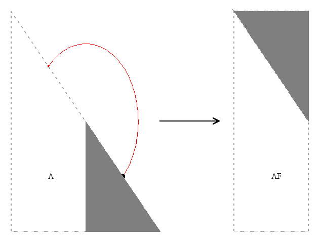
Figure 1
Figure 1 gives a graphical representation of the key idea of RFP for the particular case of a lower triangular matrix of even dimensions. In all cases the original triangular matrix of stored elements is separated into a trapezoidal part and a triangular part. The number of columns in these two parts is equal when the dimension of the matrix is even, , while the trapezoidal part has columns when . The smaller part is then transposed and fitted onto the trapezoidal part forming a rectangle. The rectangle has dimensions and , where when is even and when is odd.
For functions using RFP there is the option of storing the rectangle as described above () or its transpose (, for real a) or its conjugate transpose (, for complex a). It is useful to note that the storage ordering for Nag_RowMajor is the same as that for Nag_ColMajor with the value of switched to or vice versa.
As an example, we first consider RFP for the case with .
If , then ar holds a as follows:
For the upper trapezoid consists of the last three columns of a upper. The lower triangle consists of the transpose of the first three columns of a upper.
For the lower trapezoid consists of the first three columns of a lower. The upper triangle consists of the transpose of the last three columns of a lower.
If , then ar in both uplo cases is just the transpose of ar as defined when .
uplo
Triangle of matrix
Rectangular Full Packed matrix
Nag_Upper
Nag_Lower
Now we consider RFP for the case and .
If . ar holds a as follows:
if the upper trapezoid consists of the last three columns of a upper. The lower triangle consists of the transpose of the first two columns of a upper;
if the lower trapezoid consists of the first three columns of a lower. The upper triangle consists of the transpose of the last two columns of a lower.
If . ar in both uplo cases is just the transpose of ar as defined when .
uplo
Triangle of matrix
Rectangular Full Packed matrix
Nag_Upper
Nag_Lower
Explicitly, in the real matrix case, ar is a one-dimensional array of length and, when Nag_ColMajor, contains the elements of a as follows:
for
and ,
is stored in
, for and , and
is stored in
, for and ;
for and ,
is stored in
, for and , and
is stored in
, for and ;
for and ,
is stored in
, for and , and
is stored in
, for and ;
for and ,
is stored in
, for and , and
is stored in
, for and .
When Nag_RowMajor the above storage formulae can be used by looking up the opposite case for transr, i.e., when look up the storage order above for the cases when and vice versa.
In the case of complex matrices, the assumption is that the full matrix, if it existed, would be Hermitian. Thus, when , the triangular portion of a that is, in the real case, transposed into the notional RFP matrix is also conjugated. When the notional RFP matrix is the conjugate transpose of the corresponding RFP matrix. Explicitly, for complex a, the array ar contains the elements (or conjugated elements) of a as follows:
for
and ,
is stored in
, for and , and
is stored in
, for and ;
for and ,
is stored in
, for and , and
is stored in
, for and ;
for and ,
is stored in
, for and , and
is stored in
, for and ;
for and ,
is stored in
, for and , and
is stored in
, for and .
When Nag_RowMajor the above storage formulae can be used by looking up the opposite case for transr, i.e., when look up the storage order above for the cases when and vice versa.
3.3.4Band storage
A band matrix with subdiagonals and superdiagonals may be stored compactly in a notional two-dimensional array with rows and columns if stored column-wise or rows and columns if stored row-wise. In column-major order, elements of a column of the matrix are stored contiguously in the array, and elements of the diagonals of the matrix are stored with constant stride (i.e., in a row of the two-dimensional array). In row-major order, elements of a row of the matrix are stored contiguously in the array, and elements of a diagonal of the matrix are stored with constant stride (i.e., in a column of the two-dimensional array). These storage schemes should only be used in practice if , , although the functions in Chapters F07 and F08 work correctly for all values of and . In Chapters F07 and F08 arrays which hold matrices in band storage have names ending in .
To be precise, elements of matrix elements are stored as follows:
if , is stored in ;
if , is stored in ,
where is the stride between diagonal elements and where .
For example, when , and :
Band matrix
Band storage in array ab
The elements marked in the upper left and lower right corners of the array ab need not be set, and are not referenced by the functions.
In this example, if and ldab takes the minimum value of , then need not be set, . On the other hand, if (), then and need not be set, .
Note: when a general band matrix is supplied for factorization, space must be allowed to store an additional superdiagonals, generated by fill-in as a result of row interchanges. This means that the matrix is stored according to the above scheme, but with
superdiagonals; it also means that the principal dimension has the constraint .
Triangular band matrices are stored in the same format, with either if upper triangular, or if lower triangular.
For symmetric or Hermitian band matrices with subdiagonals or superdiagonals, only the upper or lower triangle (as specified by uplo) need be stored:
if then
if , is stored in ;
if , is stored in .
for ;
if then
if , is stored in ;
if , is stored in .
for ,
where is the stride separating diagonal matrix elements in the array ab.
For example, when and :
uplo
Hermitian band matrix
Band storage in array ab
Nag_Upper
Nag_Lower
Note that different storage schemes for band matrices are used by some functions in Chapters F01, F02, F03 and F04.
In the above example, if and , then for , ; while for , . If (), then for , ; while for , .
3.3.5Unit triangular matrices
Some functions in this chapter have an option to handle unit triangular matrices (that is, triangular matrices with diagonal elements ). This option is specified by an argument diag. If (Unit triangular), the diagonal elements of the matrix need not be stored, and the corresponding array elements are not referenced by the functions. The storage scheme for the rest of the matrix (whether conventional, packed or band) remains unchanged.
3.3.6Real diagonal elements of complex matrices
Complex Hermitian matrices have diagonal elements that are by definition purely real. In addition, complex triangular matrices which arise in Cholesky factorization are defined by the algorithm to have real diagonal elements.
If such matrices are supplied as input to functions in Chapters F07 and F08, the imaginary parts of the diagonal elements are not referenced, but are assumed to be zero. If such matrices are returned as output by the functions, the computed imaginary parts are explicitly set to zero.
3.4Parameter Conventions
3.4.1Option arguments
In addition to the order argument of type Nag_OrderType, most functions in this Chapter have one or more option arguments of various types; only options of the correct type may be supplied.
For example,
nag_lapacklin_dpotrf(Nag_RowMajor,Nag_Upper,...)
3.4.2Problem dimensions
It is permissible for the problem dimensions (for example, m in f07adc, n or nrhs in f07aec) to be passed as zero, in which case the computation (or part of it) is skipped. Negative dimensions are regarded as an error.
3.5Tables of Driver and Computational Functions
3.5.1Real matrices
Each entry gives:
the NAG function short name
the LAPACK routine name from which the NAG function long name is derived by prepending nag_.
5Auxiliary Functions Associated with Library Function Arguments
None.
6 Withdrawn or Deprecated Functions
None.
7References
Anderson E, Bai Z, Bischof C, Blackford S, Demmel J, Dongarra J J, Du Croz J J, Greenbaum A, Hammarling S, McKenney A and Sorensen D (1999) LAPACK Users' Guide (3rd Edition) SIAM, Philadelphia
Golub G H and Van Loan C F (1996) Matrix Computations (3rd Edition) Johns Hopkins University Press, Baltimore
Higham N J (1988) Algorithm 674: Fortran codes for estimating the one-norm of a real or complex matrix, with applications to condition estimation ACM Trans. Math. Software14 381–396
Wilkinson J H (1965) The Algebraic Eigenvalue Problem Oxford University Press, Oxford