hide long namesshow long names
hide short namesshow short names
Integer type:  int32  int64  nag_int  show int32  show int32  show int64  show int64  show nag_int  show nag_int

PDF version (NAG web site, 64-bit version, 64-bit version)
Chapter Contents
Chapter Introduction
NAG Toolbox

NAG Toolbox: nag_smooth_withdraw_kerndens_gauss (g10ba)

 Contents

    1  Purpose
    2  Syntax
    7  Accuracy
    9  Example

Purpose

nag_smooth_kerndens_gauss (g10ba) performs kernel density estimation using a Gaussian kernel.
Note: this function is scheduled to be withdrawn, please see g10ba in Advice on Replacement Calls for Withdrawn/Superseded Routines..

Syntax

[smooth, t, fft, ifail] = g10ba(x, window, slo, shi, usefft, fft, 'n', n, 'ns', ns)
[smooth, t, fft, ifail] = nag_smooth_withdraw_kerndens_gauss(x, window, slo, shi, usefft, fft, 'n', n, 'ns', ns)

Description

Given a sample of n observations, x1,x2,,xn, from a distribution with unknown density function, fx, an estimate of the density function, f^x, may be required. The simplest form of density estimator is the histogram. This may be defined by:
f^ x = 1nh nj ,   a + j-1 h < x < a + j h ,   j=1,2,,ns ,  
where nj is the number of observations falling in the interval a+j-1h to a+jh, a is the lower bound to the histogram and b=nsh is the upper bound. The value h is known as the window width. To produce a smoother density estimate a kernel method can be used. A kernel function, Kt, satisfies the conditions:
-Ktdt=1  and  Kt0.  
The kernel density estimator is then defined as
f^x=1nh i= 1nK x-xih .  
The choice of K is usually not important but to ease the computational burden use can be made of the Gaussian kernel defined as
Kt=12πe-t2/2.  
The smoothness of the estimator depends on the window width h. The larger the value of h the smoother the density estimate. The value of h can be chosen by examining plots of the smoothed density for different values of h or by using cross-validation methods (see Silverman (1990)).
Silverman (1982) and Silverman (1990) show how the Gaussian kernel density estimator can be computed using a fast Fourier transform (fft). In order to compute the kernel density estimate over the range a to b the following steps are required.
(i) Discretize the data to give ns equally spaced points tl with weights ξl (see Jones and Lotwick (1984)).
(ii) Compute the fft of the weights ξl to give Yl.
(iii) Compute ζl=e-12h2sl2Yl where sl=2πl/b-a.
(iv) Find the inverse fft of ζl to give f^x.
To compute the kernel density estimate for further values of h only steps (iii) and (iv) need be repeated.

References

Jones M C and Lotwick H W (1984) Remark AS R50. A remark on algorithm AS 176. Kernel density estimation using the Fast Fourier Transform Appl. Statist. 33 120–122
Silverman B W (1982) Algorithm AS 176. Kernel density estimation using the fast Fourier transform Appl. Statist. 31 93–99
Silverman B W (1990) Density Estimation Chapman and Hall

Parameters

Compulsory Input Parameters

1:     xn – double array
The n observations, xi, for i=1,2,,n.
2:     window – double scalar
h, the window width.
Constraint: window>0.0.
3:     slo – double scalar
a, the lower limit of the interval on which the estimate is calculated. For most applications slo should be at least three window widths below the lowest data point.
Constraint: slo<shi.
4:     shi – double scalar
b, the upper limit of the interval on which the estimate is calculated. For most applications shi should be at least three window widths above the highest data point.
5:     usefft – logical scalar
Must be set to false if the values of Yl are to be calculated by nag_smooth_kerndens_gauss (g10ba) and to true if they have been computed by a previous call to nag_smooth_kerndens_gauss (g10ba) and are provided in fft. If usefft=true then the arguments n, slo, shi, ns and fft must remain unchanged from the previous call to nag_smooth_kerndens_gauss (g10ba) with usefft=false.
6:     fftns – double array
If usefft=true, fft must contain the fast Fourier transform of the weights of the discretized data, ξl, for l=1,2,,ns. Otherwise fft need not be set.

Optional Input Parameters

1:     n int64int32nag_int scalar
Default: the dimension of the array x.
n, the number of observations in the sample.
Constraint: n>0.
2:     ns int64int32nag_int scalar
Default: the dimension of the array fft.
The number of points at which the estimate is calculated, ns.
Constraints:
  • ns2;
  • The largest prime factor of ns must not exceed 19, and the total number of prime factors of ns, counting repetitions, must not exceed 20.

Output Parameters

1:     smoothns – double array
The ns values of the density estimate, f^tl, for l=1,2,,ns.
2:     tns – double array
The points at which the estimate is calculated, tl, for l=1,2,,ns.
3:     fftns – double array
The fast Fourier transform of the weights of the discretized data, ξl, for l=1,2,,ns.
4:     ifail int64int32nag_int scalar
ifail=0 unless the function detects an error (see Error Indicators and Warnings).

Error Indicators and Warnings

Errors or warnings detected by the function:

Cases prefixed with W are classified as warnings and do not generate an error of type NAG:error_n. See nag_issue_warnings.

   ifail=1
On entry,n0,
orns<2,
orshislo,
orwindow0.0.
   ifail=2
On entry,nag_smooth_kerndens_gauss (g10ba) has been called with usefft=true but the function has not been called previously with usefft=false,
ornag_smooth_kerndens_gauss (g10ba) has been called with usefft=true but some of the arguments n, slo, shi, ns have been changed since the previous call to nag_smooth_kerndens_gauss (g10ba) with usefft=false.
   ifail=3
On entry, at least one prime factor of ns is greater than 19 or ns has more than 20 prime factors.
W  ifail=4
On entry, the interval given by slo to shi does not extend beyond three window widths at either extreme of the dataset. This may distort the density estimate in some cases.
   ifail=-99
An unexpected error has been triggered by this routine. Please contact NAG.
   ifail=-399
Your licence key may have expired or may not have been installed correctly.
   ifail=-999
Dynamic memory allocation failed.

Accuracy

See Jones and Lotwick (1984) for a discussion of the accuracy of this method.

Further Comments

The time for computing the weights of the discretized data is of order n, while the time for computing the fft is of order nslogns, as is the time for computing the inverse of the fft.

Example

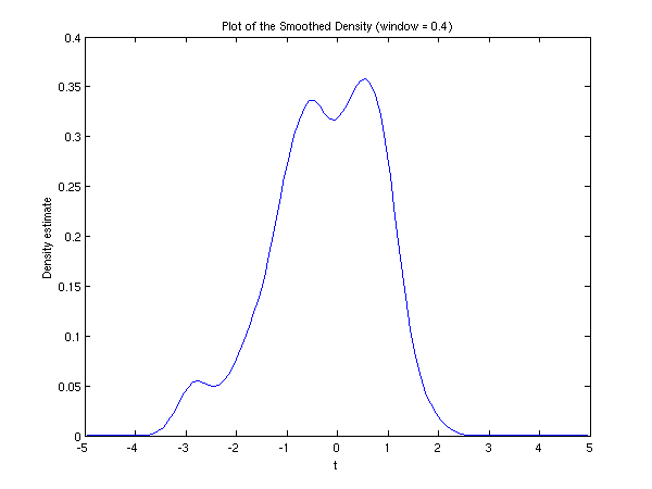
Data is read from a file and the density estimated. The first 20 values are then printed. The full estimated density function is shown in the accompanying plot.
function g10ba_example


fprintf('g10ba example results\n\n');

% sample data
x = [  0.114 -0.232 -0.570  1.853 -0.994 ...
      -0.374 -1.028  0.509  0.881 -0.453 ...
       0.588 -0.625 -1.622 -0.567  0.421 ...
      -0.475  0.054  0.817  1.015  0.608 ...
      -1.353 -0.912 -1.136  1.067  0.121 ...
      -0.075 -0.745  1.217 -1.058 -0.894 ...
       1.026 -0.967 -1.065  0.513  0.969 ...
       0.582 -0.985  0.097  0.416 -0.514 ...
       0.898 -0.154  0.617 -0.436 -1.212 ...
      -1.571  0.210 -1.101  1.018 -1.702 ...
      -2.230 -0.648 -0.350  0.446 -2.667 ...
       0.094 -0.380 -2.852 -0.888 -1.481 ...
      -0.359 -0.554  1.531  0.052 -1.715 ...
       1.255 -0.540  0.362 -0.654 -0.272 ...
      -1.810  0.269 -1.918  0.001  1.240 ...
      -0.368 -0.647 -2.282  0.498  0.001 ...
      -3.059 -1.171  0.566  0.948  0.925 ...
       0.825  0.130  0.930  0.523  0.443 ...
      -0.649  0.554 -2.823  0.158 -1.180 ...
       0.610  0.877  0.791 -0.078  1.412 ];

% Control parameters
window = 0.4;
slo    = -5;
shi    = 5;
usefft = false;
fft    = zeros(100,1);

% Perform kernel density estimation
[smooth, t, fft, ifail] = g10ba( ...
                                 x, window, slo, shi, usefft, fft);

% Display the results
fprintf('Window Width Used = %11.4e\n', window);
fprintf('Interval = (%11.4e, %11.4e)\n\n', slo, shi);
fprintf('First 20 output values:\n\n');
fprintf('      Time        Density\n');
fprintf('      Point       Estimate\n');
fprintf(' ---------------------------\n');
fprintf('%13.3e%13.3e\n', [t(1:20), smooth(1:20)]');

fig1 = figure;
plot(t,smooth);
title('Plot of the Smoothed Density (window = 0.4)');
xlabel('t');
ylabel('Density estimate');
set(gca, 'XTick', [-5:5]);

g10ba example results

Window Width Used =  4.0000e-01
Interval = (-5.0000e+00,  5.0000e+00)

First 20 output values:

      Time        Density
      Point       Estimate
 ---------------------------
   -4.950e+00    4.108e-12
   -4.850e+00    3.915e-11
   -4.750e+00    3.309e-10
   -4.650e+00    2.480e-09
   -4.550e+00    1.649e-08
   -4.450e+00    9.730e-08
   -4.350e+00    5.097e-07
   -4.250e+00    2.372e-06
   -4.150e+00    9.817e-06
   -4.050e+00    3.615e-05
   -3.950e+00    1.186e-04
   -3.850e+00    3.475e-04
   -3.750e+00    9.100e-04
   -3.650e+00    2.136e-03
   -3.550e+00    4.504e-03
   -3.450e+00    8.556e-03
   -3.350e+00    1.468e-02
   -3.250e+00    2.283e-02
   -3.150e+00    3.225e-02
   -3.050e+00    4.154e-02
g10ba_fig1.png

PDF version (NAG web site, 64-bit version, 64-bit version)
Chapter Contents
Chapter Introduction
NAG Toolbox

© The Numerical Algorithms Group Ltd, Oxford, UK. 2009–2015