PDF version (NAG web site
, 64-bit version, 64-bit version)
NAG Toolbox: nag_mv_prin_comp (g03aa)
Purpose
nag_mv_prin_comp (g03aa) performs a principal component analysis on a data matrix; both the principal component loadings and the principal component scores are returned.
Syntax
[
s,
e,
p,
v,
ifail] = g03aa(
matrix,
std,
x,
isx,
s,
nvar, 'n',
n, 'm',
m, 'wt',
wt)
[
s,
e,
p,
v,
ifail] = nag_mv_prin_comp(
matrix,
std,
x,
isx,
s,
nvar, 'n',
n, 'm',
m, 'wt',
wt)
Note: the interface to this routine has changed since earlier releases of the toolbox:
| At Mark 24: |
weight was removed from the interface; wt was made optional |
| At Mark 22: |
n was made optional |
Description
Let
be an
by
data matrix of
observations on
variables
and let the
by
variance-covariance matrix of
be
. A vector
of length
is found such that:
The variable
is known as the first principal component and gives the linear combination of the variables that gives the maximum variation. A second principal component,
, is found such that:
This gives the linear combination of variables that is orthogonal to the first principal component that gives the maximum variation. Further principal components are derived in a similar way.
The vectors
, are the eigenvectors of the matrix
and associated with each eigenvector is the eigenvalue,
. The value of
gives the proportion of variation explained by the
th principal component. Alternatively, the
's can be considered as the right singular vectors in a singular value decomposition with singular values
of the data matrix centred about its mean and scaled by
,
. This latter approach is used in
nag_mv_prin_comp (g03aa), with
where
is a diagonal matrix with elements
,
is the
by
matrix with columns
and
is an
by
matrix with
, which gives the principal component scores.
Principal component analysis is often used to reduce the dimension of a dataset, replacing a large number of correlated variables with a smaller number of orthogonal variables that still contain most of the information in the original dataset.
The choice of the number of dimensions required is usually based on the amount of variation accounted for by the leading principal components. If
principal components are selected, then a test of the equality of the remaining
eigenvalues is
which has, asymptotically, a
-distribution with
degrees of freedom.
Equality of the remaining eigenvalues indicates that if any more principal components are to be considered then they all should be considered.
Instead of the variance-covariance matrix the correlation matrix, the sums of squares and cross-products matrix or a standardized sums of squares and cross-products matrix may be used. In the last case is replaced by for a diagonal matrix with positive elements. If the correlation matrix is used, the approximation for the statistic given above is not valid.
The principal component scores, , are the values of the principal component variables for the observations. These can be standardized so that the variance of these scores for each principal component is or equal to the corresponding eigenvalue.
Weights can be used with the analysis, in which case the matrix is first centred about the weighted means then each row is scaled by an amount , where is the weight for the th observation.
References
Chatfield C and Collins A J (1980) Introduction to Multivariate Analysis Chapman and Hall
Cooley W C and Lohnes P R (1971) Multivariate Data Analysis Wiley
Hammarling S (1985) The singular value decomposition in multivariate statistics SIGNUM Newsl. 20(3) 2–25
Kendall M G and Stuart A (1969) The Advanced Theory of Statistics (Volume 1) (3rd Edition) Griffin
Morrison D F (1967) Multivariate Statistical Methods McGraw–Hill
Parameters
Compulsory Input Parameters
- 1:
– string (length ≥ 1)
-
Indicates for which type of matrix the principal component analysis is to be carried out.
- It is for the correlation matrix.
- It is for a standardized matrix, with standardizations given by s.
- It is for the sums of squares and cross-products matrix.
- It is for the variance-covariance matrix.
Constraint:
, , or .
- 2:
– string (length ≥ 1)
-
Indicates if the principal component scores are to be standardized.
- The principal component scores are standardized so that , i.e., .
- The principal component scores are unstandardized, i.e., .
- The principal component scores are standardized so that they have unit variance.
- The principal component scores are standardized so that they have variance equal to the corresponding eigenvalue.
Constraint:
, , or .
- 3:
– double array
-
ldx, the first dimension of the array, must satisfy the constraint
.
must contain the th observation for the th variable, for and .
- 4:
– int64int32nag_int array
-
indicates whether or not the
th variable is to be included in the analysis.
If
, the variable contained in the
th column of
x is included in the principal component analysis, for
.
Constraint:
for
nvar values of
.
- 5:
– double array
-
The standardizations to be used, if any.
If
, the first
elements of
s must contain the standardization coefficients, the diagonal elements of
.
Constraint:
if , , for .
- 6:
– int64int32nag_int scalar
-
, the number of variables in the principal component analysis.
Constraint:
.
Optional Input Parameters
- 1:
– int64int32nag_int scalar
-
Default:
the first dimension of the array
x.
, the number of observations.
Constraint:
.
- 2:
– int64int32nag_int scalar
-
Default:
the dimension of the arrays
isx,
s and the second dimension of the array
x. (An error is raised if these dimensions are not equal.)
, the number of variables in the data matrix.
Constraint:
.
- 3:
– double array
-
The dimension of the array
wt
must be at least
if
, and at least
otherwise
If
, the first
elements of
wt must contain the weights to be used in the principal component analysis.
If , the th observation is not included in the analysis. The effective number of observations is the sum of the weights.
If
,
wt is not referenced and the effective number of observations is
.
Constraints:
- , for ;
- the sum of weights .
Output Parameters
- 1:
– double array
-
If
,
s is unchanged on exit.
If
,
s contains the variances of the selected variables.
contains the variance of the variable in the
th column of
x if
.
If
or
,
s is not referenced.
- 2:
– double array
-
The statistics of the principal component analysis.
- The eigenvalues associated with the
th principal component, , for .
- The proportion of variation explained by the
th principal component, for .
- The cumulative proportion of variation explained by the first
th principal components, for .
- The statistics, for .
- The degrees of freedom for the statistics, for .
If ,
contains significance level for the statistic, for .
If , is returned as zero.
- 3:
– double array
-
The first
nvar columns of
p contain the principal component loadings,
. The
th column of
p contains the
nvar coefficients for the
th principal component.
- 4:
– double array
-
The first
nvar columns of
v contain the principal component scores. The
th column of
v contains the
n scores for the
th principal component.
If , any rows for which is zero will be set to zero.
- 5:
– int64int32nag_int scalar
unless the function detects an error (see
Error Indicators and Warnings).
Error Indicators and Warnings
Errors or warnings detected by the function:
Cases prefixed with W are classified as warnings and
do not generate an error of type NAG:error_n. See nag_issue_warnings.
-
-
| On entry, | , |
| or | , |
| or | , |
| or | , |
| or | , |
| or | , |
| or | , |
| or | , |
| or | , |
| or | , , or , |
| or | , , or , |
| or | or . |
-
-
| On entry, | and a value of . |
-
-
| On entry, | there are not nvar values of , |
| or | and the effective number of observations is less than . |
-
-
| On entry, | for some , when and . |
-
-
The singular value decomposition has failed to converge. This is an unlikely error exit.
- W
-
All eigenvalues/singular values are zero. This will be caused by all the variables being constant.
-
An unexpected error has been triggered by this routine. Please
contact
NAG.
-
Your licence key may have expired or may not have been installed correctly.
-
Dynamic memory allocation failed.
Accuracy
As nag_mv_prin_comp (g03aa) uses a singular value decomposition of the data matrix, it will be less affected by ill-conditioned problems than traditional methods using the eigenvalue decomposition of the variance-covariance matrix.
Further Comments
None.
Example
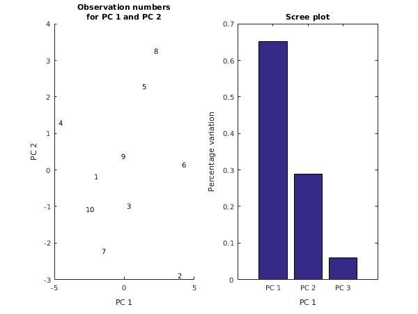
A dataset is taken from
Cooley and Lohnes (1971), it consists of ten observations on three variables. The unweighted principal components based on the variance-covariance matrix are computed and the principal component scores requested. The principal component scores are standardized so that they have variance equal to the corresponding eigenvalue.
Open in the MATLAB editor:
g03aa_example
function g03aa_example


fprintf('g03aa example results\n\n');

x    = [7, 4, 3;
	4, 1, 8;
	6, 3, 5;
	8, 6, 1;
	8, 5, 7;
	7, 2, 9;
	5, 3, 3;
	9, 5, 8;
	7, 4, 5;
	8, 2, 2];
n    = size(x,2);

matrix = 'V';
std  = 'E';
isx  = ones(n,1,'int64');
s    = zeros(n,1);
nvar = int64(n);

[s, e, p, v, ifail] = g03aa( ...
			     matrix, std, x, isx, s, nvar);

fprintf('Eigenvalues  Percentage  Cumulative     Chisq      DF     Sig\n');
fprintf('              variation   variation\n\n');
fprintf('%11.4f%12.4f%12.4f%10.4f%8.1f%8.4f\n',e');
fprintf('\n');

mtitle = 'Principal component loadings';
matrix = 'General';
diag   = ' ';

[ifail] = x04ca( ...
                 matrix, diag, p, mtitle);

fprintf('\n');
mtitle = 'Principal component scores';
[ifail] = x04ca( ...
                 matrix, diag, v, mtitle);

fig1 = figure;
subplot(1,2,1);
xlabel('PC 1');
ylabel('PC 2');
title({'Observation numbers', 'for PC 1 and PC 2'});
axis([-5 5 -3 4]);
for j = 1:size(x,1)
  ch = sprintf('%d',j);
  text(v(j,1),v(j,2),ch);
end
subplot(1,2,2);
bar(e(:,2));
ax = gca;
ax.XTickLabel = {'PC 1','PC 2','PC 3'};
xlabel('PC 1');
ylabel('Percentage variation');
title('Scree plot');
g03aa example results

Eigenvalues  Percentage  Cumulative     Chisq      DF     Sig
              variation   variation

     8.2739      0.6515      0.6515    8.6127     5.0  0.1255
     3.6761      0.2895      0.9410    4.1183     2.0  0.1276
     0.7499      0.0590      1.0000    0.0000     0.0  0.0000

 Principal component loadings
          1       2       3
 1  -0.1376  0.6990 -0.7017
 2  -0.2505  0.6609  0.7075
 3   0.9583  0.2731  0.0842

 Principal component scores
              1          2          3
  1     -2.1514    -0.1731     0.1068
  2      3.8042    -2.8875     0.5104
  3      0.1532    -0.9869     0.2694
  4     -4.7065     1.3015     0.6517
  5      1.2938     2.2791     0.4492
  6      4.0993     0.1436    -0.8031
  7     -1.6258    -2.2321     0.8028
  8      2.1145     3.2512    -0.1684
  9     -0.2348     0.3730     0.2751
 10     -2.7464    -1.0689    -2.0940
PDF version (NAG web site
, 64-bit version, 64-bit version)
© The Numerical Algorithms Group Ltd, Oxford, UK. 2009–2015