PDF version (NAG web site
, 64-bit version, 64-bit version)
NAG Toolbox: nag_pde_2d_laplace (d03ea)
Purpose
nag_pde_2d_laplace (d03ea) solves Laplace's equation in two dimensions for an arbitrary domain bounded internally or externally by one or more closed contours, given the value of either the unknown function or its normal derivative (into the domain) at each point of the boundary.
Syntax
[
phi,
phid,
alpha,
ifail] = d03ea(
stage1,
ext,
dorm,
p,
q,
x,
y,
phi,
phid,
alpha, 'n',
n, 'n1p1',
n1p1)
[
phi,
phid,
alpha,
ifail] = nag_pde_2d_laplace(
stage1,
ext,
dorm,
p,
q,
x,
y,
phi,
phid,
alpha, 'n',
n, 'n1p1',
n1p1)
Description
nag_pde_2d_laplace (d03ea) uses an integral equation method, based upon Green's formula, which yields the solution, , within the domain, given its value or that of its normal derivative at each point of the boundary (except possibly at a finite number of discrete points). The solution is obtained in two stages. The first, which is executed once only, determines the complementary boundary values, i.e., , where its normal derivative is known and vice versa. The second stage is entered once for each point at which the solution is required.
The boundary is divided into a number of intervals in each of which
and its normal derivative are approximated by constants. Of these half are evaluated by applying the given boundary conditions at one ‘nodal’ point within each interval while the remainder are determined (in stage
) by solving a set of simultaneous linear equations. Here this is achieved by means of auxiliary function
nag_lapack_dgels (f08aa), which will yield the least squares solution of an overdetermined system of equations as well as the unique solution of a square nonsingular system.
In exterior domains the solution behaves as as tends to infinity, where is a constant, is the total integral of the normal derivative around the boundary and is the radial distance from the origin of coordinates. For the Neumann problem (when the normal derivative is given along the whole boundary) is fixed by the boundary conditions whilst is chosen by you. However, for a Dirichlet problem (when is given along the whole boundary) or for a mixed problem, stage produces a value of for which ; then as tends to infinity the solution tends to the constant .
References
Symm G T and Pitfield R A (1974) Solution of Laplace's equation in two dimensions NPL Report NAC 44 National Physical Laboratory
Parameters
Compulsory Input Parameters
- 1:
– logical scalar
-
Indicates whether the function call is for stage
of the computation as defined in
Description.
- The call is for stage .
- The call is for stage .
- 2:
– logical scalar
-
The form of the domain. If , the domain is unbounded. Otherwise the domain is an interior one.
- 3:
– logical scalar
-
The form of the boundary conditions. If , then the problem is a Dirichlet or mixed boundary value problem. Otherwise it is a Neumann problem.
- 4:
– double scalar
- 5:
– double scalar
-
To stage
,
p and
q must specify the
and
coordinates respectively of a point at which the solution is required.
When
stage1 is
true,
p and
q are ignored.
- 6:
– double array
- 7:
– double array
-
The
and
coordinates respectively of points on the one or more closed contours which define the domain of the problem.
Note: each contour is described in such a manner that the subscripts of the coordinates increase when the domain is kept on the left. The final point on each contour coincides with the first and, if a further contour is to be described, the coordinates of this point are repeated in the arrays. In this way each interval is defined by three points, the second of which (the nodal point) always has an even subscript. In the case of the interior Neumann problem, the outermost boundary contour must be given first, if there is more than one.
- 8:
– double array
-
For stage
,
phi must contain the nodal values of
or its normal derivative (into the domain) as prescribed in each interval. For stage
it must retain its output values from stage
.
- 9:
– double array
-
For stage , must hold the value or accordingly as contains a value of or its normal derivative, for . For stage it must retain its output values from stage .
- 10:
– double scalar
-
For stage
, the use of
alpha depends on the nature of the problem:
- if , alpha need not be set;
- if and , alpha must contain the prescribed constant (see Description);
- if and , alpha must contain an appropriate value (often zero) for the integral of around the outermost boundary.
For stage
, on every call
alpha must contain the value returned at stage
.
Optional Input Parameters
- 1:
– int64int32nag_int scalar
-
Default:
the dimension of the arrays
phi,
phid. (An error is raised if these dimensions are not equal.)
The number of intervals into which the boundary is divided (see
Accuracy and
Further Comments).
- 2:
– int64int32nag_int scalar
-
Default:
the dimension of the arrays
x,
y. (An error is raised if these dimensions are not equal.)
The value , where denotes the number of closed contours which make up the boundary.
Output Parameters
- 1:
– double array
-
From stage , it contains the constants which approximate in each interval. It remains unchanged on exit from stage .
- 2:
– double array
-
From stage
,
phid contains the constants which approximate the normal derivative of
in each interval. It remains unchanged on exit from stage
.
- 3:
– double scalar
-
From stage
:
- if , alpha contains ;
- if and alpha is unchanged;
- if and alpha contains a computed estimate for .
From stage
:
- alpha contains the computed value of at the point (p,q).
- 4:
– int64int32nag_int scalar
unless the function detects an error (see
Error Indicators and Warnings).
Error Indicators and Warnings
Errors or warnings detected by the function:
-
-
Invalid tolerance used in an internal call to an auxiliary function:
- Indicates too large a tolerance.
- Indicates too small a tolerance.
Note: this error is only possible in stage 1, and the circumstances under which it may occur cannot be foreseen. In the event of a failure, it is suggested that you change the scale of the domain of the problem and apply the function again.
-
-
Incorrect rank obtained by an auxiliary function; contains the computed rank.
-
An unexpected error has been triggered by this routine. Please
contact
NAG.
-
Your licence key may have expired or may not have been installed correctly.
-
Dynamic memory allocation failed.
Accuracy
The accuracy of the computed solution depends upon how closely and its normal derivative may be approximated by constants in each interval of the boundary and upon how well the boundary contours are represented by polygons with vertices at the selected points
, for .
Consequently, in general, the accuracy increases as the boundary is subdivided into smaller and smaller intervals and by comparing solutions for successive subdivisions one may obtain an indication of the error in these solutions.
Alternatively, since the point of maximum error always lies on the boundary of the domain, an estimate of the error may be obtained by computing at a sufficient number of points on the boundary where the true solution is known. The latter method (not applicable to the Neumann problem) is most useful in the case where alone is prescribed on the boundary (the Dirichlet problem).
Further Comments
The time taken for stage 1, which is executed once only, is roughly proportional to
, being dominated by the time taken to compute the coefficients. The time for each stage
application is proportional to
n.
The intervals into which the boundary is divided need not be of equal lengths.
For many practical problems useful results may be obtained with to intervals per boundary contour.
Example
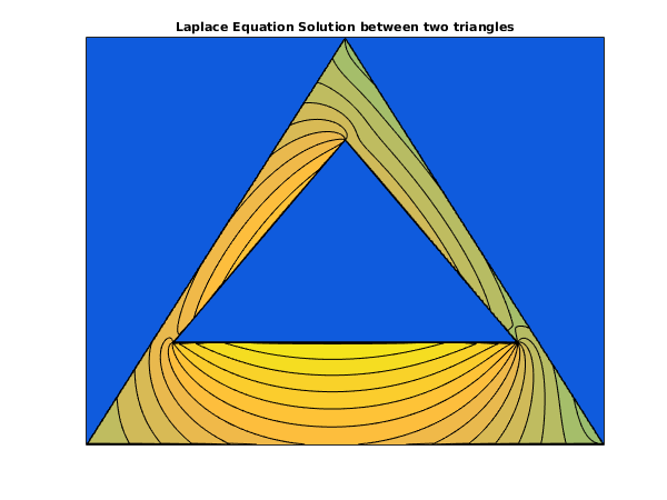
An interior Neumann problem to solve Laplace's equation in the domain bounded externally by the triangle with vertices , and , and internally by the triangle with vertices , () and , given that the normal derivative of the solution is zero on each side of each triangle and, for uniqueness that the total integral of around the outer triangle is (the length of the contour).
This trivial example has the obvious solution throughout the domain. However it provides a useful illustration of data input for a doubly-connected domain. The solution is computed at one corner of each triangle and at one point inside the domain.
The program is written to handle any of the different types of problem that the function can solve. The array dimensions must be increased for larger problems.
Open in the MATLAB editor:
d03ea_example
function d03ea_example
fprintf('d03ea example results\n\n');
stage1 = true;
ext = false;
dorm = false;
p = 0;
q = 0;
x = [ 3.0; 1.5; 0.0; -1.5; -3.0; 0.0; 3.0;
3.0;
2.0; 0.0; -2.0; -1.0; 0.0; 1.0; 2.0];
y = [ 0.0; 2.0; 4.0; 2.0; 0.0; 0.0; 0.0;
0.0;
1.0; 1.0; 1.0; 2.0; 3.0; 2.0; 1.0];
phi(1:6) = [3, 4, 4, 5, 4, 3];
phid(1:6) = [0, 0, 0, 0, 0, 0];
alpha = 12;
[phi, phid, alpha, ifail] = ...
d03ea( ...
stage1, ext, dorm, p, q, x, y, phi, phid, alpha);
stage1 = false;
phisol = zeros(401,601);
solmin = 1.e10;
solmax = -1.0e10;
i = 0;
for xx = -3:0.01:3
i = i + 1;
j = 0;
xl = 3-abs(xx);
y1 = (4/3)*xl;
for yy = 0:0.01:4
j = j + 1;
if ( (yy<=y1) && ((yy<=1) || (yy>=xl)));
[phi, phid, sol, ifail] = ...
d03ea( ...
stage1, ext, dorm, xx, yy, x, y, phi, phid, alpha);
phisol(j,i) = sol;
solmax = max(solmax,sol);
solmin = min(solmin,sol);
end
end
end
fprintf('The maximum value of solution = %8.3f\n',solmax);
fprintf('The minimum value of solution = %8.3f\n',solmin);
fig1 = figure;
contourf(phisol,[solmin:-1,1,2:0.2:solmax]);
title('Laplace Equation Solution between two triangles');
set(gca,'XTick',[],'XTickLabel',[],'YTick',[],'YTickLabel',[]);
d03ea example results

The maximum value of solution =    5.430
The minimum value of solution =   -2.979
PDF version (NAG web site
, 64-bit version, 64-bit version)
© The Numerical Algorithms Group Ltd, Oxford, UK. 2009–2015