PDF version (NAG web site
, 64-bit version, 64-bit version)
NAG Toolbox: nag_ode_bvp_coll_nth (d02ja)
Purpose
nag_ode_bvp_coll_nth (d02ja) solves a regular linear two-point boundary value problem for a single th-order ordinary differential equation by Chebyshev series using collocation and least squares.
Syntax
Description
nag_ode_bvp_coll_nth (d02ja) calculates the solution of a regular two-point boundary value problem for a single
th-order linear ordinary differential equation as a Chebyshev series in the interval
. The differential equation
is defined by
cf, and the boundary conditions at the points
and
are defined by
bc.
You specify the degree of Chebyshev series required,
, and the number of collocation points,
kp. The function sets up a system of linear equations for the Chebyshev coefficients, one equation for each collocation point and one for each boundary condition. The boundary conditions are solved exactly, and the remaining equations are then solved by a least squares method. The result produced is a set of coefficients for a Chebyshev series solution of the differential equation on an interval normalized to
.
nag_fit_1dcheb_eval2 (e02ak) can be used to evaluate the solution at any point on the interval
– see
Example for an example.
nag_fit_1dcheb_deriv (e02ah) followed by
nag_fit_1dcheb_eval2 (e02ak) can be used to evaluate its derivatives.
References
Picken S M (1970) Algorithms for the solution of differential equations in Chebyshev-series by the selected points method Report Math. 94 National Physical Laboratory
Parameters
Compulsory Input Parameters
- 1:
– int64int32nag_int scalar
-
, the order of the differential equation.
Constraint:
.
- 2:
– function handle or string containing name of m-file
-
cf defines the differential equation (see
Description). It must return the value of a function
at a given point
, where, for
,
is the coefficient of
in the equation, and
is the right-hand side.
[result] = cf(j, x)
Input Parameters
- 1:
– int64int32nag_int scalar
-
The index of the function to be evaluated.
- 2:
– double scalar
-
The point at which is to be evaluated.
Output Parameters
- 1:
– double scalar
-
The value of at the given point .
- 3:
– function handle or string containing name of m-file
-
bc defines the boundary conditions, each of which has the form
or
. The boundary conditions may be specified in any order.
[j, rhs] = bc(ii)
Input Parameters
- 1:
– int64int32nag_int scalar
-
The index of the boundary condition to be defined.
Output Parameters
- 1:
– int64int32nag_int scalar
-
Must be set to
if the boundary condition is
, and to
if it is
.
j must not be set to the same value
for two different values of
ii.
- 2:
– double scalar
-
Must be set to the value .
- 4:
– double scalar
- 5:
– double scalar
-
The left- and right-hand boundaries, and , respectively.
Constraint:
.
- 6:
– int64int32nag_int scalar
-
The number of coefficients to be returned in the Chebyshev series representation of the solution (hence the degree of the polynomial approximation is ).
Constraint:
.
- 7:
– int64int32nag_int scalar
-
The number of collocation points to be used.
Constraint:
.
Optional Input Parameters
None.
Output Parameters
- 1:
– double array
-
The computed Chebyshev coefficients; that is, the computed solution is:
where
is the
th Chebyshev polynomial of the first kind, and
denotes that the first coefficient,
, is halved.
- 2:
– int64int32nag_int scalar
unless the function detects an error (see
Error Indicators and Warnings).
Error Indicators and Warnings
Errors or warnings detected by the function:
-
-
| On entry, | , |
| or | , |
| or | , |
| or | . |
-
-
| On entry, | (insufficient workspace). |
-
-
Either the boundary conditions are not linearly independent (that is, in
bc the variable
j is set to the same value
for two different values of
ii), or the rank of the matrix of equations for the coefficients is less than the number of unknowns. Increasing
kp may overcome this latter problem.
-
-
The least squares function
nag_linsys_real_gen_lsqsol (f04am) has failed to correct the first approximate solution (see
nag_linsys_real_gen_lsqsol (f04am)).
-
An unexpected error has been triggered by this routine. Please
contact
NAG.
-
Your licence key may have expired or may not have been installed correctly.
-
Dynamic memory allocation failed.
Accuracy
The Chebyshev coefficients are determined by a stable numerical method. The accuracy of the approximate solution may be checked by varying the degree of the polynomial and the number of collocation points (see
Further Comments).
Further Comments
The time taken by nag_ode_bvp_coll_nth (d02ja) depends on the complexity of the differential equation, the degree of the polynomial solution, and the number of matching points.
The collocation points in the interval are chosen to be the extrema of the appropriate shifted Chebyshev polynomial. If , then the least squares solution reduces to the solution of a system of linear equations, and true collocation results.
The accuracy of the solution may be checked by repeating the calculation with different values of
k1 and with
kp fixed but
. If the Chebyshev coefficients decrease rapidly (and consistently for various
k1 and
kp), the size of the last two or three gives an indication of the error. If the Chebyshev coefficients do not decay rapidly, it is likely that the solution cannot be well-represented by Chebyshev series. Note that the Chebyshev coefficients are calculated for the interval
.
Systems of regular linear differential equations can be solved using
nag_ode_bvp_coll_sys (d02jb). It is necessary before using
nag_ode_bvp_coll_sys (d02jb) to write the differential equations as a first-order system. Linear systems of high-order equations in their original form, singular problems, and, indirectly, nonlinear problems can be solved using
nag_ode_bvp_coll_nth_comp (d02tg).
Example
This example solves the equation
with boundary conditions
We use
,
and
, and
and
, so that the different Chebyshev series may be compared. The solution for
and
is evaluated by
nag_fit_1dcheb_eval2 (e02ak) at nine equally spaced points over the interval
.
Open in the MATLAB editor:
d02ja_example
function d02ja_example
fprintf('d02ja example results\n\n');
n = int64(2);
k1max = 8;
kpmax = 15;
lw = 2*(kpmax+n)*(k1max+1)+7*k1max;
x0 = -1;
x1 = 1;
c = zeros(1,kpmax);
p = zeros(1,kpmax);
fprintf(' KP K1 Chebyshev coefficients\n');
for kp = int64(10:5:kpmax)
for k1 = int64(4:2:k1max)
[c, ifail] = d02ja(n, @cf, @bc, x0, x1, k1, kp);
fprintf('%4d ',kp, k1);
for kind = 1:k1
fprintf('%8.4f ',c(kind));
if mod(kind, 6) == 0 && kind ~= k1
fprintf('\n ');
end
end
fprintf('\n');
end
end
fprintf('\n');
k1 = int64(8);
k1m1 = int64(k1-1);
m = 9;
ia1 = int64(1);
xarray = zeros(k1,1);
yarray = zeros(k1,1);
fprintf('Last computed solution evaluated at %1d equally spaced points\n\n', m);
fprintf(' X Y\n');
for i = 1:m
x = (x0*double(m-i)+x1*double(i-1))/double(m-1);
[y, ifail] = e02ak(k1m1, x0, x1, c, ia1, x);
fprintf('%8.4f %8.4f \n',x,y);
xarray(i) = x;
yarray(i) = y;
end
fig1 = figure;
display_plot(xarray, yarray)
function [j, rhs] = bc(i)
rhs = 0;
if (i == 1)
j = int64(1);
else
j = int64(-1);
end
function result = cf(j, x)
if (j == 2)
result = 0;
else
result = 1;
end
function display_plot(x, y)
plot(x, y, '-+');
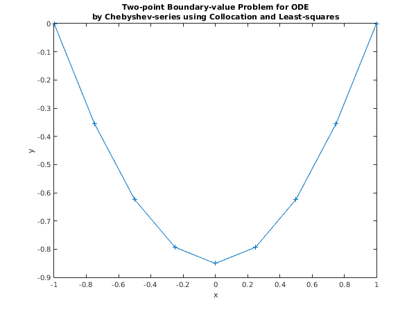
title({'Two-point Boundary-value Problem for ODE',...
'by Chebyshev-series using Collocation and Least-squares'})
xlabel('x');
ylabel('y');
d02ja example results

  KP   K1   Chebyshev coefficients
  10    4  -0.6108   -0.0000    0.3054    0.0000
  10    6  -0.8316   -0.0000    0.4246    0.0000   -0.0088   -0.0000
  10    8  -0.8325   -0.0000    0.4253    0.0000   -0.0092    0.0000
            0.0001   -0.0000
  15    4  -0.6174   -0.0000    0.3087    0.0000
  15    6  -0.8316   -0.0000    0.4246    0.0000   -0.0088   -0.0000
  15    8  -0.8325   -0.0000    0.4253    0.0000   -0.0092   -0.0000
            0.0001    0.0000

Last computed solution evaluated at 9 equally spaced points

    X         Y
 -1.0000    0.0000
 -0.7500   -0.3542
 -0.5000   -0.6242
 -0.2500   -0.7933
  0.0000   -0.8508
  0.2500   -0.7933
  0.5000   -0.6242
  0.7500   -0.3542
  1.0000    0.0000
PDF version (NAG web site
, 64-bit version, 64-bit version)
© The Numerical Algorithms Group Ltd, Oxford, UK. 2009–2015