PDF version (NAG web site
, 64-bit version, 64-bit version)
NAG Toolbox: nag_ode_bvp_shoot_bval (d02ha)
Purpose
nag_ode_bvp_shoot_bval (d02ha) solves a two-point boundary value problem for a system of ordinary differential equations, using a Runge–Kutta–Merson method and a Newton iteration in a shooting and matching technique.
Syntax
[
u,
soln,
w,
ifail] = d02ha(
u,
v,
a,
b,
tol,
fcn,
m1, 'n',
n)
[
u,
soln,
w,
ifail] = nag_ode_bvp_shoot_bval(
u,
v,
a,
b,
tol,
fcn,
m1, 'n',
n)
Description
nag_ode_bvp_shoot_bval (d02ha) solves a two-point boundary value problem for a system of
ordinary differential equations in the range
. The system is written in the form:
and the derivatives
are evaluated by
fcn. Initially,
boundary values of the variables
must be specified, some at
and some at
. You must supply estimates of the remaining
boundary values (called parameters below); the function corrects these by a form of Newton iteration. It also calculates the complete solution on an equispaced mesh if required.
Starting from the known and estimated values of
at
, the function integrates the equations from
to
(using a Runge–Kutta–Merson method). The differences between the values of
at
from integration and those specified initially should be zero for the true solution. (These differences are called residuals below.) The function uses a generalized Newton method to reduce the residuals to zero, by calculating corrections to the estimated boundary values. This process is repeated iteratively until convergence is obtained, or until the function can no longer reduce the residuals. See
Hall and Watt (1976) for a simple discussion of shooting and matching techniques.
References
Hall G and Watt J M (ed.) (1976) Modern Numerical Methods for Ordinary Differential Equations Clarendon Press, Oxford
Parameters
Compulsory Input Parameters
- 1:
– double array
-
must be set to the known or estimated value of at and must be set to the known or estimated value of at , for .
- 2:
– double array
-
must be set to if is a known value and to if is an estimated value, for and .
Constraint:
precisely of the must be set to , i.e., precisely of the must be known values, and these must not be all at or all at .
- 3:
– double scalar
-
, the initial point of the interval of integration.
- 4:
– double scalar
-
, the final point of the interval of integration.
- 5:
– double scalar
-
Must be set to a small quantity suitable for:
| (a) |
testing the local error in during integration, |
| (b) |
testing for the convergence of at , |
| (c) |
calculating the perturbation in estimated boundary values for , which are used to obtain the approximate derivatives of the residuals for use in the Newton iteration. |
You are advised to check your results by varying
tol.
Constraint:
.
- 6:
– function handle or string containing name of m-file
-
fcn must evaluate the functions
(i.e., the derivatives
), for
, at a general point
.
[f] = fcn(x, y)
Input Parameters
- 1:
– double scalar
-
, the value of the argument.
- 2:
– double array
-
, for , the value of the argument.
Output Parameters
- 1:
– double array
-
The values of
, for .
- 7:
– int64int32nag_int scalar
-
A value which controls output.
- The final solution is not evaluated.
- The final values of
at interval are calculated and stored in the array soln by columns, starting with values at stored in , for .
Constraint:
.
Optional Input Parameters
- 1:
– int64int32nag_int scalar
-
Default:
the first dimension of the arrays
u,
v. (An error is raised if these dimensions are not equal.)
, the number of equations.
Constraint:
.
Output Parameters
- 1:
– double array
-
The known values unaltered, and corrected values of the estimates, unless an error has occurred. If an error has occurred,
u contains the known values and the latest values of the estimates.
- 2:
– double array
-
The solution when .
- 3:
– double array
-
.
If , , or ,
, for , contains the solution at the point where the integration fails and the point of failure is returned in .
- 4:
– int64int32nag_int scalar
unless the function detects an error (see
Error Indicators and Warnings).
Error Indicators and Warnings
Errors or warnings detected by the function:
-
-
One or more of the arguments
v,
n,
m1,
sdw, or
tol is incorrectly set.
-
-
The step length for the integration is too short whilst calculating the residual (see
Further Comments).
-
-
No initial step length could be chosen for the integration whilst calculating the residual.
Note: or
can occur due to choosing too small a value for
tol or due to choosing the wrong direction of integration. Try varying
tol and interchanging
and
. These error exits can also occur for very poor initial estimates of the unknown initial values and, in extreme cases, because
nag_ode_bvp_shoot_bval (d02ha) cannot be used to solve the problem posed.
-
-
As for but the error occurred when calculating the Jacobian of the derivatives of the residuals with respect to the parameters.
-
-
As for but the error occurred when calculating the derivatives of the residuals with respect to the parameters.
-
-
The calculated Jacobian has an insignificant column.
Note: ,
or
usually indicate a badly scaled problem. You may vary the size of
tol or change to one of the more general functions
nag_ode_bvp_shoot_genpar (d02hb) or
nag_ode_bvp_shoot_genpar_algeq (d02sa) which afford more control over the calculations.
-
-
The linear algebra function (
nag_lapack_dgesvd (f08kb)) used has failed. This error exit should not occur and can be avoided by changing the estimated initial values.
-
-
The Newton iteration has failed to converge.
Note: can indicate poor initial estimates or a very difficult problem. Consider varying
tol if the residuals are small in the monitoring output. If the residuals are large try varying the initial estimates.
-
-
-
-
-
-
Indicates that a serious error has occurred in an internal call. Check all array subscripts and function argument lists in calls to nag_ode_bvp_shoot_bval (d02ha). Seek expert help.
-
An unexpected error has been triggered by this routine. Please
contact
NAG.
-
Your licence key may have expired or may not have been installed correctly.
-
Dynamic memory allocation failed.
Accuracy
If the process converges, the accuracy to which the unknown parameters are determined is usually close to that specified by you; the solution, if requested, may be determined to a required accuracy by varying
tol.
Further Comments
The time taken by nag_ode_bvp_shoot_bval (d02ha) depends on the complexity of the system, and on the number of iterations required. In practice, integration of the differential equations is by far the most costly process involved.
Wherever it occurs in the function, the error argument
tol is used in ‘mixed’ form; that is
tol always occurs in expressions of the form
. Though not ideal for every application, it is expected that this mixture of absolute and relative error testing will be adequate for most purposes.
You are strongly recommended to set
ifail to obtain self-explanatory error messages, and also monitoring information about the course of the computation. You may select the channel numbers on which this output is to appear by calls of
nag_file_set_unit_error (x04aa) (for error messages) or
nag_file_set_unit_advisory (x04ab) (for monitoring information) – see
Example for an example. Otherwise the default channel numbers will be used. The monitoring information produced at each iteration includes the current parameter values, the residuals and
-norms: a basic norm and a current norm. At each iteration the aim is to find parameter values which make the current norm less than the basic norm. Both these norms should tend to zero as should the residuals. (They would all be zero if the exact parameters were used as input.) For more details, you may consult the specification of
nag_ode_bvp_shoot_genpar_algeq (d02sa), and especially the description of the argument
monit there.
The computing time for integrating the differential equations can sometimes depend critically on the quality of the initial estimates. If it seems that too much computing time is required and, in particular, if the values of the residuals printed by the monitoring function are much larger than the expected values of the solution at
, then the coding of
fcn should be checked for errors. If no errors can be found, an independent attempt should be made to improve the initial estimates. In practical problems it is not uncommon for the differential equation to have a singular point at one or both ends of the range. Suppose
is a singular point; then the derivatives
in
(1) (in
Description) cannot be evaluated at
, usually because one or more of the expressions for
give overflow. In such a case it is necessary for you to take
a short distance away from the singularity, and to find values for
at the new value of
(e.g., use the first one or two terms of an analytical (power series) solution). You should experiment with the new position of
; if it is taken too close to the singular point, the derivatives
will be inaccurate, and the function may sometimes fail with
or
or, in extreme cases, with an overflow condition. A more general treatment of singular solutions is provided by the function
nag_ode_bvp_shoot_genpar (d02hb).
Another difficulty which often arises in practice is the case when one end of the range,
say, is at infinity. You must approximate the end point by taking a finite value for
, which is obtained by estimating where the solution will reach its asymptotic state. The estimate can be checked by repeating the calculation with a larger value of
. If
is very large, and if the matching point is also at
, the numerical solution may suffer a considerable loss of accuracy in integrating across the range, and the program may fail with
or
. (In the former case, solutions from all initial values at
are tending to the same curve at infinity.) The simplest remedy is to try to solve the equations with a smaller value of
, and then to increase
in stages, using each solution to give boundary value estimates for the next calculation. For problems where some terms in the asymptotic form of the solution are known,
nag_ode_bvp_shoot_genpar (d02hb) will be more successful.
If the unknown quantities are not boundary values, but are eigenvalues or the length of the range or some other parameters occurring in the differential equations,
nag_ode_bvp_shoot_genpar (d02hb) may be used.
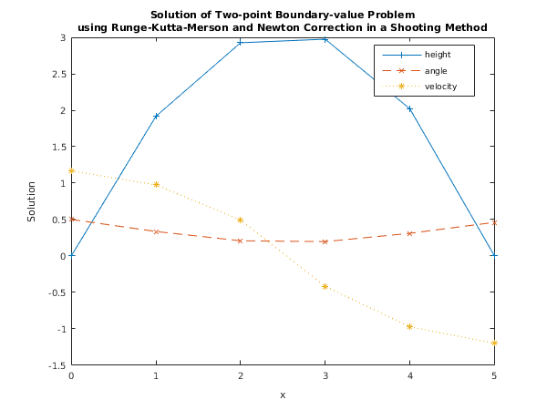
Example
This example finds the angle at which a projectile must be fired for a given range.
The differential equations are:
with the following boundary conditions:
The remaining boundary conditions are estimated as:
We write
,
,
. To check the accuracy of the results the problem is solved twice with
.
and
respectively. Note the call to
nag_file_set_unit_advisory (x04ab) before the call to
nag_ode_bvp_shoot_bval (d02ha).
Open in the MATLAB editor:
d02ha_example
function d02ha_example
fprintf('d02ha example results\n\n');
u = [0, 0; 0.5, 0.46; 1.15, -1.2];
v = [0, 0; 0, 1; 1, 1];
a = 0;
b = 5;
m1 = 6;
n = 3;
ykeep = zeros(m1,3);
xkeep = zeros(1,m1);
for id = 3:4
tol = 5*10^(-id);
[uOut, soln, w, ifail] = d02ha(u, v, a, b, tol, @fcn, int64(m1));
if (ifail ~= 0)
error('Warning: d02ha returned with ifail = %d ',ifail);
else
fprintf('Results with tol = %1.3e\n\n',tol);
fprintf('X-value and final solution\n\n');
for i = 1:m1
disp((sprintf('%d %8.4f %8.4f %8.4f', i-1,...
soln(1,i),soln(2,i),soln(3,i))));
ykeep(i,1) = soln(1,i);
ykeep(i,2) = soln(2,i);
ykeep(i,3) = soln(3,i);
xkeep(i) = i-1;
end
end
disp(' ');
end
fig1 = figure;
display_plot(xkeep, ykeep)
function f = fcn(x,y)
f = zeros(3,1);
f(1) = tan(y(3));
f(2) = -0.032*tan(y(3))/y(2) - 0.02*y(2)/cos(y(3));
f(3) = -0.032/y(2)^2;
function display_plot(xkeep, ykeep)
plot(xkeep, ykeep(:,1), '-+',...
xkeep, ykeep(:,2), '--x',...
xkeep, ykeep(:,3), ':*');
title({'Solution of Two-point Boundary-value Problem',...
['using Runge-Kutta-Merson and Newton Correction in a ', ...
'Shooting Method']});
xlabel('x');
ylabel('Solution');
legend('height','angle','velocity','location','Best');
d02ha example results

Results with tol = 5.000e-03

X-value and final solution

0     0.0000     0.5000     1.1685
1     1.9197     0.3341     0.9752
2     2.9304     0.2066     0.4917
3     2.9767     0.1956    -0.4228
4     2.0258     0.3093    -0.9754
5    -0.0005     0.4598    -1.2020

Results with tol = 5.000e-04

X-value and final solution

0     0.0000     0.5000     1.1681
1     1.9177     0.3343     0.9749
2     2.9280     0.2070     0.4929
3     2.9769     0.1955    -0.4194
4     2.0210     0.3095    -0.9751
5    -0.0000     0.4597    -1.2014
PDF version (NAG web site
, 64-bit version, 64-bit version)
© The Numerical Algorithms Group Ltd, Oxford, UK. 2009–2015