g13ek:: Time Series Analysis (NAG Toolbox)

Given

{\hat{x}}_{0}

, an initial estimate of the state and

P_{0}

and initial estimate of the state covariance matrix, the UKF can be described as follows:

(a)

Generate a set of sigma points (see Sigma Points):

X_{t}

= [{\hat{x}}_{t - 1} {\hat{x}}_{t - 1} + γ \sqrt{P_{t - 1}} {\hat{x}}_{t - 1} - γ \sqrt{P_{t - 1}}]

(1)

(b)

Evaluate the known model function

F

F_{t}

= F (X_{t})

(2)

The function

F

is assumed to accept the

m_{x} \times n

matrix,

X_{t}

and return an

m_{x} \times n

matrix,

F_{t}

. The columns of both

X_{t}

and

F_{t}

correspond to different possible states. The notation

F_{t, i}

is used to denote the

i

th column of

F_{t}

, hence the result of applying

F

to the

i

th possible state.

(c)

Time Update:

${\hat{x}}_{t}^{_}$	$= \sum_{i = 1}^{n} W_{i}^{m} F_{t, i}$	(3)
$P_{t}^{_}$	$= \sum_{i = 1}^{n} W_{i}^{c} (F_{t, i} - {\hat{x}}_{t}^{_}) {(F_{t, i} - {\hat{x}}_{t}^{_})}^{T} + Σ_{x}$	(4)

(d)

Redraw another set of sigma points (see Sigma Points):

Y_{t}

= [{\hat{x}}_{t}^{_} {\hat{x}}_{t}^{_} + γ \sqrt{P_{t}^{_}} {\hat{x}}_{t}^{_} - γ \sqrt{P_{t}^{_}}]

(5)

(e)

Evaluate the known model function

H

H_{t}

= H (Y_{t})

(6)

The function

H

is assumed to accept the

m_{x} \times n

matrix,

Y_{t}

and return an

m_{y} \times n

matrix,

H_{t}

. The columns of both

Y_{t}

and

H_{t}

correspond to different possible states. As above

H_{t, i}

is used to denote the

i

th column of

H_{t}

(f)

Measurement Update:

${\hat{y}}_{t}$	$= \sum_{i = 1}^{n} W_{i}^{m} H_{t, i}$	(7)
$P_{y y_{t}}$	$= \sum_{i = 1}^{n} W_{i}^{c} (H_{t, i} - {\hat{y}}_{t}) {(H_{t, i} - {\hat{y}}_{t})}^{T} + Σ_{y}$	(8)
$P_{x y_{t}}$	$= \sum_{i = 1}^{n} W_{i}^{c} (F_{t, i} - {\hat{x}}_{t}^{_}) {(H_{t, i} - {\hat{y}}_{t})}^{T}$	(9)
$K_{t}$	$= P_{x y_{t}} P_{y y_{t}}^{- 1}$	(10)
${\hat{x}}_{t}$	$= {\hat{x}}_{t}^{_} + K_{t} (y_{t} - {\hat{y}}_{t})$	(11)
$P_{t}$	$= P_{t}^{_} - K_{t} P_{y y_{t}} K_{t}^{T}$	(12)

Sigma Points

When calculating the weighted sample mean and covariance matrix two sets of weights are required, one used when calculating the weighted sample mean, denoted

W^{m}

and one used when calculated the weighted sample covariance matrix, denoted

W^{c}

. The weights and multiplier,

γ

, are constructed as follows:

\begin{matrix} λ & = α^{2} (L + κ) - L \\ γ & = \sqrt{L + λ} \\ W_{i}^{m} & = \{\begin{matrix} \frac{λ}{L + λ} & i = 1 \\ \frac{1}{2 (L + λ)} & i = 2, 3, \dots, 2 L + 1 \end{matrix} \\ W_{i}^{c} & = \{\begin{matrix} \frac{λ}{L + λ} + 1 - α^{2} + β & i = 1 \\ \frac{1}{2 (L + λ)} & i = 2, 3, \dots, 2 L + 1 \end{matrix} \end{matrix}

where, usually

L = m

and

α, β

and

κ

are constants. The total number of sigma points,

n

, is given by

2 L + 1

. The constant

α

is usually set to somewhere in the range

10^{- 4} \leq α \leq 1

and for a Gaussian distribution, the optimal values of

κ

and

β

are

3 - L

and

2

respectively.

References

Parameters

Compulsory Input Parameters

Optional Input Parameters

Output Parameters

Error Indicators and Warnings

Accuracy

Further Comments

Example

This example implements the following nonlinear state space model, with the state vector

x

and state update function

F

given by:

\begin{matrix} m_{x} & = 3 \\ x_{t + 1} & = {(\begin{matrix} ξ_{t + 1} & η_{t + 1} & θ_{t + 1} \end{matrix})}^{T} \\ = F (x_{t}) + v_{t} \\ = x_{t} + (\begin{array}{l} \cos θ_{t} & - \sin θ_{t} & 0 \\ \sin θ_{t} & \cos θ_{t} & 0 \\ 0 & 0 & 1 \end{array}) (\begin{array}{l} 0.5 r & 0.5 r \\ 0 & 0 \\ r / d & - r / d \end{array}) (\begin{array}{l} ϕ_{R t} \\ ϕ_{L t} \end{array}) + v_{t} \end{matrix}

where

r

and

d

are known constants and

ϕ_{R t}

and

ϕ_{L t}

are time-dependent knowns. The measurement vector

y

and measurement function

H

is given by:

\begin{matrix} m_{y} & = 2 \\ y_{t} & = {(δ_{t}, α_{t})}^{T} \\ = H (x_{t}) + u_{t} \\ = (\begin{matrix} Δ - ξ_{t} \cos A - η_{t} \sin A \\ θ_{t} - A \end{matrix}) + u_{t} \end{matrix}

where

A

and

Δ

are known constants. The initial values,

x_{0}

and

P_{0}

, are given by

\begin{matrix} x_{0} & = & (\begin{matrix} 0 \\ 0 \\ 0 \end{matrix}), & P_{0} & = & (\begin{matrix} 0.1 & 0 & 0 \\ 0 & 0.1 & 0 \\ 0 & 0 & 0.1 \end{matrix}) \end{matrix}

and the Cholesky factorizations of the error covariance matrices,

L_{x}

and

L_{x}

\begin{matrix} \begin{matrix} L_{x} & = & (\begin{matrix} 0.1 & 0 & 0 \\ 0 & 0.1 & 0 \\ 0 & 0 & 0.1 \end{matrix}) \end{matrix}, & \begin{matrix} L_{y} & = & (\begin{matrix} 0.01 & 0 \\ 0 & 0.01 \end{matrix}) \end{matrix} \end{matrix}

function g13ek_example


fprintf('g13ek example results\n\n');

% Cholesky factorisation of the covariance matrix for
% the process noise
lx = 0.1 * eye(3);

% Cholesky factorisation of the covariance matrix for
% the observation noise
ly = 0.01 * eye(2);

% Initial state vector
ix = zeros(size(lx,1),1);
x = ix;

% Cholesky factorisation of the initial state covariance matrix
st = 0.1 * eye(3);

% Constant terms in the state space model
r = 3;
d = 4;
Delta = 5.814;
A = 0.464;

% Observed data, y = (delta, alpha)
y = [5.2620 4.3470 3.8180 2.7060 1.8780 0.6840 0.7520 ...
     0.4640 0.5970 0.8420 1.4120 1.5270 2.3990 2.6610 3.3270;
     5.9230 5.7830 6.1810 0.0850 0.4420 0.8360 1.3000 ...
     1.7000 1.7810 2.0400 2.2860 2.8200 3.1470 3.5690 3.6590];

% Number of time points to run the system for
ntime = size(y,2);

% phi_r and phi_l (these are the same across all time points in
% this example)
phi_r = ones(ntime,1) * 0.4;
phi_l = ones(ntime,1) * 0.1;

mx = numel(x);

% Reserve some space to hold the state
cx = zeros(mx,ntime);

% Loop over each time point
for t = 1:ntime

  % Observed data at time point t
  y_t = y(:,t);
  phi_rt = phi_r(t);
  phi_lt = phi_l(t);

  % Store the information required by f and h in a cell array
  user = {Delta;A;r;d;phi_rt;phi_lt};

  % Update the state and its covariance matrix
  [x,st,user,ifail] = g13ek( ...
                             y_t,lx,ly,@f,@h,x,st,'user',user);

  % Store the current state
  cx(:,t) = x(:);
end

% Print the results
ttext = ['  Time  ' blanks(ceil((11*mx- 16)/2)) ' Estimate of State' ...
                    blanks(ceil((11*mx -16)/2))];
fprintf('%s\n',ttext);
ttext(:) = '-';
fprintf('%s\n',ttext);
for t = 1:ntime
  fprintf('  %3d   ', t);
  fprintf(' %10.3f', cx(1:mx,t));
  fprintf('\n');
end

fprintf('\nEstimate of Cholesky Factorisation of the State\n');
fprintf('Covariance Matrix at the Last Time Point\n');
for i=1:mx
  for j=1:i
    fprintf(' %10.2e',st(i,j));
  end
  fprintf('\n');
end

% Plot the results
fig1 = figure;

% calculate and plot the position and facing of the robot as if there
% were no slippage in the wheels
pos_no_slippage(:,1) = ix;
rot_mat = [r/2 r/2; 0 0;r/d -r/d];
for t=1:ntime
  v_r = rot_mat * [phi_r(t); phi_l(t)];
  theta = pos_no_slippage(3,t);
  T = [cos(theta) -sin(theta) 0; sin(theta) cos(theta) 0; 0 0 1];
  pos_no_slippage(:,t+1) = pos_no_slippage(:,t) + T*v_r;
end

% formula (of the form y = a + b x) for the position of the wall
b = -cos(A) / sin(A);
a = Delta * (sin(A) + cos(A)^2/sin(A));

% actual position and facing of the robot
% (this would usually be unknown, but this example
% is based on a simulation and hence we know the answer)
pos_actual = [0.000 0.617 1.590 2.192 ...
              3.238 3.947 4.762 4.734 ...
              4.529 3.955 3.222 2.209 ...
              2.047 1.137 0.903 0.443;
              0.000 0.000 0.101 0.079 ...
              0.474 0.908 1.947 1.850 ...
              2.904 3.757 4.675 5.425 ...
              5.492 5.362 5.244 4.674;
              0.000 0.103 0.036 0.361 ...
              0.549 0.906 1.299 1.763 ...
              2.164 2.245 2.504 2.749 ...
              3.284 3.610 4.033 4.123];

% produce the plot
h(1) = plot_robot(pos_no_slippage,'s','green','green');
hold on
h(2) = plot_robot(pos_actual,'c','red','red');
h(3) = plot_robot([zeros(3,1) cx],'c','blue','none');
hold off

% Add reference line for the wall
yl = ylim;
line([(yl(1) - a)/b (yl(2) - a) / b],yl,'Color','black');
xlim([-0.5 7]);

% Add title
title({'{\bf g13ek Example Plot}', 
       'Illustration of Position and Orientation',
       ' of Hypothetical Robot'});

% Add legend
label = ['Initial' 'Actual' 'Updated'];
h(4) = legend(h,'Initial','Actual','Updated','Location','NorthEast');
set(h(4),'FontSize',get(h(4),'FontSize')*0.8);

% Add text to indicate wall
text(4.6,3.9,'Wall','Rotation',-63);



function [fxt,user,info] = f(xt,user,info)
  r = user{3};
  d = user{4};
  phi_rt = user{5};
  phi_lt = user{6};

  t1 = 0.5*r*(phi_rt+phi_lt);
  t3 = (r/d)*(phi_rt-phi_lt);

  fxt(1,:) = xt(1,:) + cos(xt(3,:))*t1;
  fxt(2,:) = xt(2,:) + sin(xt(3,:))*t1;
  fxt(3,:) = xt(3,:) + t3;

  % Set info nonzero to terminate execution for any reason.
  info = int64(0);

function [hyt,user,info] = h(yt,user,info)
  Delta = user{1};
  A = user{2};

  hyt(1,:) = Delta - yt(1,:)*cos(A) - yt(2,:)*sin(A);
  hyt(2,:) = yt(3,:) - A;

  % Make sure that the theta is in the same range as the observed
  % data, which in this case is [0, 2*pi)
  hyt(2,(hyt(2,:) < 0)) = hyt(2,(hyt(2,:) < 0)) + 2 * pi;

  % Set info nonzero to terminate execution for any reason.
  info = int64(0);

function [h] =  plot_robot(x,symbol,colour,fill)
  alen = 0.3;
  h = scatter(x(1,:),x(2,:),60,colour,symbol,'MarkerFaceColor',fill);
  aend = [x(1,:)+alen*cos(x(3,:)); x(2,:)+alen*sin(x(3,:))];
  line([x(1,:); aend(1,:)],[x(2,:); aend(2,:)],'Color',colour);

g13ek example results

  Time            Estimate of State         
--------------------------------------------
    1         0.664     -0.092      0.104
    2         1.598      0.081      0.314
    3         2.128      0.213      0.378
    4         3.134      0.674      0.660
    5         3.809      1.181      0.906
    6         4.730      2.000      1.298
    7         4.429      2.474      1.762
    8         4.357      3.246      2.162
    9         3.907      3.852      2.246
   10         3.360      4.398      2.504
   11         2.552      4.741      2.750
   12         2.191      5.193      3.281
   13         1.309      5.018      3.610
   14         1.071      4.894      4.031
   15         0.618      4.322      4.124

Estimate of Cholesky Factorisation of the State
Covariance Matrix at the Last Time Point
   1.92e-01
  -3.82e-01   2.22e-02
   1.58e-06   2.23e-07   9.95e-03

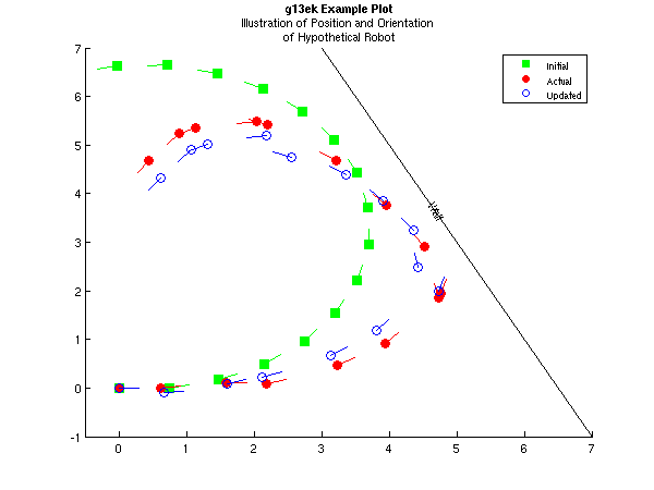
The example described above can be thought of relating to the movement of a hypothetical robot. The unknown state,

x

, is the position of the robot (with respect to a reference frame) and facing, with

(ξ, η)

giving the

x

and

y

coordinates and

θ

the angle (with respect to the

x

-axis) that the robot is facing. The robot has two drive wheels, of radius

r

on an axle of length

d

. During time period

t

the right wheel is believed to rotate at a velocity of

ϕ_{R t}

and the left at a velocity of

ϕ_{L t}

. In this example, these velocities are fixed with

ϕ_{R t} = 0.4

and

ϕ_{L t} = 0.1

. The state update function,

F

, calculates where the robot should be at each time point, given its previous position. However, in reality, there is some random fluctuation in the velocity of the wheels, for example, due to slippage. Therefore the actual position of the robot and the position given by equation

F

will differ.

NAG Toolbox: nag_tsa_kalman_unscented_state (g13ek)

▸▿ Contents

Purpose

Syntax

Description

Unscented Kalman Filter Algorithm

Sigma Points

References

Parameters

Compulsory Input Parameters

Optional Input Parameters

Output Parameters

Error Indicators and Warnings

Accuracy

Further Comments

Example

References

Haykin S (2001) Kalman Filtering and Neural Networks John Wiley and Sons
Julier S J (2002) The scaled unscented transformation Proceedings of the 2002 American Control Conference (Volume 6) 4555–4559
Julier S J and Uhlmann J K (1997a) A consistent, debiased method for converting between polar and Cartesian coordinate systems Proceedings of AeroSense97, International Society for Optics and Phonotonics 110–121
Julier S J and Uhlmann J K (1997b) A new extension of the Kalman Filter to nonlinear systems International Symposium for Aerospace/Defense, Sensing, Simulation and Controls (Volume 3) 26