e02dd:: Curve and Surface Fitting (NAG Toolbox)

The spline is given in the B-spline representation

s (x, y) = \sum_{i = 1}^{n_{x} - 4} \sum_{j = 1}^{n_{y} - 4} c_{i j} M_{i} (x) N_{j} (y),

(1)

where

M_{i} (x)

and

N_{j} (y)

denote normalized cubic B-splines, the former defined on the knots

λ_{i}

λ_{i + 4}

and the latter on the knots

μ_{j}

μ_{j + 4}

. For further details, see Hayes and Halliday (1974) for bicubic splines and de Boor (1972) for normalized B-splines.

The total numbers

n_{x}

and

n_{y}

of these knots and their values

λ_{1}, \dots, λ_{n_{x}}

and

μ_{1}, \dots, μ_{n_{y}}

are chosen automatically by the function. The knots

λ_{5}, \dots, λ_{n_{x} - 4}

and

μ_{5}, \dots, μ_{n_{y} - 4}

are the interior knots; they divide the approximation domain

[x_{\min}, x_{\max}] \times [y_{\min}, y_{\max}]

into

(n_{x} - 7) \times (n_{y} - 7)

subpanels

[λ_{i}, λ_{i + 1}] \times [μ_{j}, μ_{j + 1}]

, for

i = 4, 5, \dots, n_{x} - 4

and

j = 4, 5, \dots, n_{y} - 4

. Then, much as in the curve case (see nag_fit_1dspline_auto (e02be)), the coefficients

c_{i j}

are determined as the solution of the following constrained minimization problem:

minimize

η,

(2)

subject to the constraint

θ = \sum_{r = 1}^{m} ε_{r}^{2} \leq S

(3)

where:	$η$	is a measure of the (lack of) smoothness of $s (x, y)$ . Its value depends on the discontinuity jumps in $s (x, y)$ across the boundaries of the subpanels. It is zero only when there are no discontinuities and is positive otherwise, increasing with the size of the jumps (see Dierckx (1981b) for details).
	$ε_{r}$	denotes the weighted residual $w_{r} (f_{r} - s (x_{r}, y_{r}))$ ,
and	$s$	is a non-negative number to be specified by you.

By means of the argument

s

, ‘the smoothing factor’, you will then control the balance between smoothness and closeness of fit, as measured by the sum of squares of residuals in (3). If

s

is too large, the spline will be too smooth and signal will be lost (underfit); if

s

is too small, the spline will pick up too much noise (overfit). In the extreme cases the method would return an interpolating spline

(θ = 0)

s

were set to zero, and returns the least squares bicubic polynomial

(η = 0)

s

is set very large. Experimenting with

s

-values between these two extremes should result in a good compromise. (See Choice of for advice on choice of

s

.) Note however, that this function, unlike nag_fit_1dspline_auto (e02be) and nag_fit_2dspline_grid (e02dc), does not allow

s

to be set exactly to zero: to compute an interpolant to scattered data, nag_interp_2d_scat (e01sa) or nag_interp_2d_scat_shep (e01sg) should be used.

References

Parameters

Compulsory Input Parameters

Optional Input Parameters

Output Parameters

Error Indicators and Warnings

Accuracy

On successful exit, the approximation returned is such that its weighted sum of squared residuals fp is equal to the smoothing factor

s

, up to a specified relative tolerance of

0.001

– except that if

n_{x} = 8

and

n_{y} = 8

, fp may be significantly less than

s

: in this case the computed spline is simply the least squares bicubic polynomial approximation of degree

3

, i.e., a spline with no interior knots.

Further Comments

Timing

Choice of s

If the weights have been correctly chosen (see Weighting of data points in the E02 Chapter Introduction), the standard deviation of

w_{r} f_{r}

would be the same for all

r

, equal to

σ

, say. In this case, choosing the smoothing factor

s

in the range

σ^{2} (m \pm \sqrt{2 m})

, as suggested by Reinsch (1967), is likely to give a good start in the search for a satisfactory value. Otherwise, experimenting with different values of

s

will be required from the start.

In that case, in view of computation time and memory requirements, it is recommended to start with a very large value for

s

and so determine the least squares bicubic polynomial; the value returned for fp, call it

{fp}_{0}

, gives an upper bound for

s

. Then progressively decrease the value of

s

to obtain closer fits – say by a factor of

10

in the beginning, i.e.,

s = {fp}_{0} / 10

s = {fp}_{0} / 100

, and so on, and more carefully as the approximation shows more details.

The number of knots of the spline returned, and their location, generally depend on the value of

s

and on the behaviour of the function underlying the data. However, if nag_fit_2dspline_sctr (e02dd) is called with

start ='W'

, the knots returned may also depend on the smoothing factors of the previous calls. Therefore if, after a number of trials with different values of

s

and

start ='W'

, a fit can finally be accepted as satisfactory, it may be worthwhile to call nag_fit_2dspline_sctr (e02dd) once more with the selected value for

s

but now using

start ='C'

. Often, nag_fit_2dspline_sctr (e02dd) then returns an approximation with the same quality of fit but with fewer knots, which is therefore better if data reduction is also important.

Choice of nxest and nyest

The number of knots may also depend on the upper bounds nxest and nyest. Indeed, if at a certain stage in nag_fit_2dspline_sctr (e02dd) the number of knots in one direction (say

n_{x}

) has reached the value of its upper bound (nxest), then from that moment on all subsequent knots are added in the other

(y)

direction. This may indicate that the value of nxest is too small. On the other hand, it gives you the option of limiting the number of knots the function locates in any direction. For example, by setting

nxest = 8

(the lowest allowable value for nxest), you can indicate that you want an approximation which is a simple cubic polynomial in the variable

x

Restriction of the approximation domain

The fit obtained is not defined outside the rectangle

[λ_{4}, λ_{n_{x} - 3}] \times [μ_{4}, μ_{n_{y} - 3}]

. The reason for taking the extreme data values of

x

and

y

for these four knots is that, as is usual in data fitting, the fit cannot be expected to give satisfactory values outside the data region. If, nevertheless, you require values over a larger rectangle, this can be achieved by augmenting the data with two artificial data points

(a, c, 0)

and

(b, d, 0)

with zero weight, where

[a, b] \times [c, d]

denotes the enlarged rectangle.

Outline of method used

First suitable knot sets are built up in stages (starting with no interior knots in the case of a cold start but with the knot set found in a previous call if a warm start is chosen). At each stage, a bicubic spline is fitted to the data by least squares and

θ

, the sum of squares of residuals, is computed. If

θ > s

, a new knot is added to one knot set or the other so as to reduce

θ

at the next stage. The new knot is located in an interval where the fit is particularly poor. Sooner or later, we find that

θ \leq s

and at that point the knot sets are accepted. The function then goes on to compute a spline which has these knot sets and which satisfies the full fitting criterion specified by (2) and (3). The theoretical solution has

θ = s

. The function computes the spline by an iterative scheme which is ended when

θ = s

within a relative tolerance of

0.001

. The main part of each iteration consists of a linear least squares computation of special form, done in a similarly stable and efficient manner as in nag_fit_2dspline_panel (e02da). As there also, the minimal least squares solution is computed wherever the linear system is found to be rank-deficient.

An exception occurs when the function finds at the start that, even with no interior knots (

N = 8

), the least squares spline already has its sum of squares of residuals

\leq s

. In this case, since this spline (which is simply a bicubic polynomial) also has an optimal value for the smoothness measure

η

, namely zero, it is returned at once as the (trivial) solution. It will usually mean that

s

has been chosen too large.

Evaluation of Computed Spline

The values of the computed spline at the points

(x_{r}, y_{r})

, for

r = 1, 2, \dots, n

, may be obtained in the double array ff (see nag_fit_2dspline_evalv (e02de)), of length at least

n

, by the following call:

[ff, ifail] = e02de(x, y, lamda, mu, c);

where

N = n

and the coordinates

x_{r}

y_{r}

are stored in

X (k)

Y (k)

. PX and PY have the same values as nx and ny as output from nag_fit_2dspline_sctr (e02dd), and LAMDA, MU and C have the same values as lamda, mu and c output from nag_fit_2dspline_sctr (e02dd). WRK is a double workspace array of length at least

PY - 4

, and IWRK is an integer workspace array of length at least

PY - 4

To evaluate the computed spline on a

k_{x}

k_{y}

rectangular grid of points in the

x

y

plane, which is defined by the

x

coordinates stored in

X (q)

, for

q = 1, 2, \dots, k_{x}

, and the

y

coordinates stored in

Y (r)

, for

r = 1, 2, \dots, k_{y}

, returning the results in the double array ff (see nag_fit_2dspline_evalm (e02df)) which is of length at least

mx \times my

, the following call may be used:

[fg, ifail] = e02df(tx, ty, lamda, mu, c);

where

KX = k_{x}

KY = k_{y}

. LAMDA, MU and C have the same values as lamda, mu and c output from nag_fit_2dspline_sctr (e02dd). WRK is a double workspace array of length at least

LWRK = \min (nwrk1, nwrk2)

, where

nwrk1 = KX \times 4 + PX

and

nwrk2 = KY \times 4 + PY

. IWRK is an integer workspace array of length at least

LIWRK = KY + PY - 4

nwrk1 \geq nwrk2

, or

KX + PX - 4

otherwise.

Example

function e02dd_example


fprintf('e02dd example results\n\n');

% Data to fit
d = [11.16   1.24  22.15; 
     12.85   3.06  22.11; 
     19.85  10.72   7.97; 
     19.72   1.39  16.83; 
     15.91   7.74  15.30; 
      0.00  20.00  34.60; 
     20.87  20.00   5.74; 
      3.45  12.78  41.24; 
     14.26  17.87  10.74; 
     17.43   3.46  18.60; 
     22.80  12.39   5.47; 
      7.58   1.98  29.87; 
     25.00  11.87   4.40; 
      0.00   0.00  58.20; 
      9.66  20.00   4.73; 
      5.22  14.66  40.36; 
     17.25  19.57   6.43; 
     25.00   3.87   8.74; 
     12.13  10.79  13.71; 
     22.23   6.21  10.25; 
     11.52   8.53  15.74; 
     15.20   0.00  21.60; 
      7.54  10.69  19.31; 
     17.32  13.78  12.11; 
      2.14  15.03  53.10; 
      0.51   8.37  49.43; 
     22.69  19.63   3.25; 
      5.47  17.13  28.63; 
     21.67  14.36   5.52; 
      3.31   0.33  44.08];
x = d(:,1);
y = d(:,2);
f = d(:,3);
w = ones(size(x));

start = 'C';
s     = 10;
nx    = int64(0);
lamda = zeros(14,1);
ny    = int64(0);
mu    = zeros(14,1);
wrk   = zeros(11016, 1);
[nx, lamda, ny, mu, c, fp, rank, wrk, ifail] = ...
e02dd( ...
       start, x, y, f, w, s, nx, lamda, ny, mu, wrk);

% Print details of spline
fprintf('\nCalling with smoothing factor S = %5.2f\n', s);
fprintf('Rank deficiency = %4d\n\n',(nx-4)*(ny-4)-rank);
fprintf('Knots:   lamda      mu\n');
for j = 4:max(nx,ny)-3
  if j<=min(nx,ny)-3
    fprintf('%4d%10.4f%10.4f\n', j, lamda(j), mu(j));
  elseif j<=nx-3
    fprintf('%4d%10.4f\n', j, lamda(j));
  else
    fprintf('%4d%20.4f\n', j, mu(j));
  end
end

cp = c(1:(ny-4)*(nx-4));
cp = reshape(cp,[ny-4,nx-4]);
fprintf('\nB-spline coefficients:\n');
disp(cp);

fprintf('Weighted sum of squared residuals = %7.4f\n', fp);
if fp==0
  fprintf('(The spline is an interpolating spline)\n');
elseif nx==8 && ny==8
  fprintf('(The spline is the weighted least-squares bi-cubic polynomial)\n');
end
fprintf('\n');

% Evaluate spline on mesh
mx = [3:21];
my = [2:17];
[ff, ifail] = e02df( ...
                     mx, my, lamda(1:nx), mu(1:ny), c);

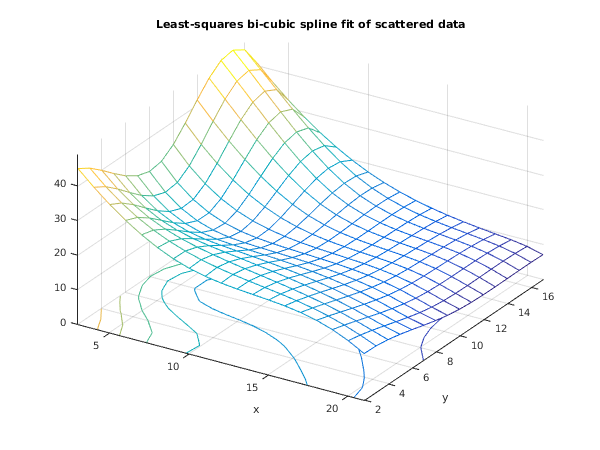
fig1 = figure;
ff = reshape(ff,[16,19]);
meshc(mx,my,ff);
xlabel('x');
ylabel('y');
title('Least-squares bi-cubic spline fit of scattered data');
view(32,40);

e02dd example results


Calling with smoothing factor S = 10.00
Rank deficiency =    0

Knots:   lamda      mu
   4    0.0000    0.0000
   5    9.7575    9.0008
   6   18.2582   20.0000
   7   25.0000

B-spline coefficients:
   58.1559   46.3067    6.0058   31.9987    5.8554  -23.7779
   63.7813   46.7449   33.3668   18.2980   14.3600   15.9518
   40.8392  -33.7898    5.1688   13.0954   -4.1317   19.3683
   75.4362  111.9175    6.9393   17.3287    7.0928  -13.2436
   34.6068  -42.6140   25.2015   -1.9641   10.3721   -9.0871

Weighted sum of squared residuals = 10.0021

On entry,	$start \neq'C'$ or $'W'$ ,
or	the number of data points with nonzero weight $< 16$ ,
or	$s \leq 0.0$ ,
or	$nxest < 8$ ,
or	$nyest < 8$ ,
or	$lwrk < (7 \times u \times v + 25 \times w) \times (w + 1) + 2 \times (u + v + 4 \times m) + 23 \times w + 56$ , where $u = nxest - 4$ , $v = nyest - 4$ and $w = \max (u, v)$ ,
or	$liwrk < m + 2 \times (nxest - 7) \times (nyest - 7)$ .

NAG Toolbox: nag_fit_2dspline_sctr (e02dd)

▸▿ Contents

Purpose

Syntax

Description

References

Parameters

Compulsory Input Parameters

Optional Input Parameters

Output Parameters

Error Indicators and Warnings

Accuracy

Further Comments

Timing

Choice of s

Choice of nxest and nyest

Restriction of the approximation domain

Outline of method used

Evaluation of Computed Spline

Example

References

de Boor C (1972) On calculating with B-splines J. Approx. Theory 6 50–62
Dierckx P (1981a) An improved algorithm for curve fitting with spline functions Report TW54 Department of Computer Science, Katholieke Univerciteit Leuven
Dierckx P (1981b) An algorithm for surface fitting with spline functions IMA J. Numer. Anal. 1 267–283
Hayes J G and Halliday J (1974) The least squares fitting of cubic spline surfaces to general data sets J. Inst. Math. Appl. 14 89–103
Peters G and Wilkinson J H (1970) The least squares problem and pseudo-inverses Comput. J. 13 309–316
Reinsch C H (1967) Smoothing by spline functions Numer. Math. 10 177–183