NAG Toolbox: nag_smooth_kerndens_gauss (g10bb)

Purpose

Syntax

Description

References

Parameters

Compulsory Input Parameters

1:     $\mathrm{x}\left(\mathbf{n}\right)$ – double array

$x_{\mathit{i}}$, for $\mathit{i}=1,2,\dots ,n$.

If $\mathbf{fcall}=0$, x must be unchanged since the last call to nag_smooth_kerndens_gauss2 (g10bb).

2:     $\mathrm{fcall}$ – int64int32nag_int scalar

If $\mathbf{fcall}=1$ then the values of $Y_l$ are to be calculated by this call to nag_smooth_kerndens_gauss2 (g10bb), otherwise it is assumed that the values of $Y_l$ were calculated by a previous call to this routine and the relevant information is stored in rcomm.

Constraint: $\mathbf{fcall}=0$ or $1$.

3:     $\mathrm{rcomm}\left(\mathbf{ns}+20\right)$ – double array

Communication array, used to store information between calls to nag_smooth_kerndens_gauss2 (g10bb).

If $\mathbf{fcall}=0$, rcomm must be unchanged since the last call to nag_smooth_kerndens_gauss2 (g10bb).

Optional Input Parameters

1:     $\mathrm{n}$ – int64int32nag_int scalar

Default: the dimension of the array x.

$n$, the number of observations in the sample.

If $\mathbf{fcall}=0$, n must be unchanged since the last call to nag_smooth_kerndens_gauss2 (g10bb).

Constraint: $\mathbf{n}>0$.

2:     $\mathrm{wtype}$ – int64int32nag_int scalar

Suggested value: $\mathbf{wtype}=2$ and $\mathbf{window}=1.0$.

Default: $2$

How the window width, $h$, is to be calculated:

$\mathbf{wtype}=1$

$h$ is supplied in window.

$\mathbf{wtype}=2$

$h$ is to be calculated from the data, with

$$h=m\times \left(\frac{0.9\times \min \left(q_{75}-q_{25},\sigma \right)}{n^{0.2}}\right)$$

where $q_{75}-q_{25}$ is the inter-quartile range and $\sigma$ the standard deviation of the sample, $x$, and $m$ is a multipler supplied in window. The $25\%$ and $75\%$ quartiles, $q_{25}$ and $q_{75}$, are calculated using nag_stat_quantiles (g01am). This is the "rule-of-thumb" suggested by Silverman (1990).

Constraint: $\mathbf{wtype}=1$ or $2$.

3:     $\mathrm{window}$ – double scalar

Suggested value: $\mathbf{window}=1.0$ and $\mathbf{wtype}=2$.

Default: $1.0$

If $\mathbf{wtype}=1$, then $h$, the window width. Otherwise, $m$, the multiplier used in the calculation of $h$.

Constraint: $\mathbf{window}>0.0$.

4:     $\mathrm{slo}$ – double scalar

Suggested value: $\mathbf{slo}=3.0$ and $\mathbf{shi}=0.0$ which would cause $a$ and $b$ to be set $3$ window widths below and above the lowest and highest data points respectively.

Default: $3.0$

If $\mathbf{slo}<\mathbf{shi}$ then $a$, the lower limit of the interval on which the estimate is calculated. Otherwise, $a$ and $b$, the lower and upper limits of the interval, are calculated as follows:

$$\begin{array}{ccc}a& =& \underset{i}{\min }\left\{x_i\right\}-\mathbf{slo}\times h\\ b& =& \underset{i}{\max }\left\{x_i\right\}+\mathbf{slo}\times h\end{array}$$

where $h$ is the window width.

For most applications $a$ should be at least three window widths below the lowest data point.

If $\mathbf{fcall}=0$, slo must be unchanged since the last call to nag_smooth_kerndens_gauss2 (g10bb).

5:     $\mathrm{shi}$ – double scalar

Default: $0.0$

If $\mathbf{slo}<\mathbf{shi}$ then $b$, the upper limit of the interval on which the estimate is calculated. Otherwise a value for $b$ is calculated from the data as stated in the description of slo and the value supplied in shi is not used.

For most applications $b$ should be at least three window widths above the highest data point.

If $\mathbf{fcall}=0$, shi must be unchanged since the last call to nag_smooth_kerndens_gauss2 (g10bb).

6:     $\mathrm{ns}$ – int64int32nag_int scalar

Default: $512$

$n_s$, the number of points at which the estimate is calculated.

If $\mathbf{fcall}=0$, ns must be unchanged since the last call to nag_smooth_kerndens_gauss2 (g10bb).

Constraints:

• $\mathbf{ns}\ge 2$;
• The largest prime factor of ns must not exceed $19$, and the total number of prime factors of ns, counting repetitions, must not exceed $20$.

Output Parameters

1:     $\mathrm{window}$ – double scalar

Suggested value: $\mathbf{window}=1.0$ and $\mathbf{wtype}=2$.

Default: $1.0$

$h$, the window width actually used.

2:     $\mathrm{slo}$ – double scalar

Suggested value: $\mathbf{slo}=3.0$ and $\mathbf{shi}=0.0$ which would cause $a$ and $b$ to be set $3$ window widths below and above the lowest and highest data points respectively.

Default: $3.0$

$a$, the lower limit actually used.

3:     $\mathrm{shi}$ – double scalar

Default: $0.0$

$b$, the upper limit actually used.

4:     $\mathrm{smooth}\left(\mathbf{ns}\right)$ – double array

$\hat{f}\left(t_{\mathit{l}}\right)$, for $\mathit{l}=1,2,\dots ,n_s$, the $n_s$ values of the density estimate.

5:     $\mathrm{t}\left(\mathbf{ns}\right)$ – double array

$t_{\mathit{l}}$, for $\mathit{l}=1,2,\dots ,n_s$, the points at which the estimate is calculated.

6:     $\mathrm{rcomm}\left(\mathbf{ns}+20\right)$ – double array

The last ns elements of rcomm contain the fast Fourier transform of the weights of the discretized data, that is $\mathbf{rcomm}\left(\mathit{l}+20\right)=Y_{\mathit{l}}$, for $\mathit{l}=1,2,\dots ,n_s$.

7:     $\mathrm{ifail}$ – int64int32nag_int scalar

$\mathbf{ifail}=\mathbf{0}$ unless the function detects an error (see Error Indicators and Warnings).

Error Indicators and Warnings

Cases prefixed with W are classified as warnings and do not generate an error of type NAG:error_n. See nag_issue_warnings.

   $\mathbf{ifail}=11$

Constraint: $\mathbf{n}>0$.

   $\mathbf{ifail}=12$

Constraint: if $\mathbf{fcall}=0$, n must be unchanged since previous call.

   $\mathbf{ifail}=31$

Constraint: $\mathbf{wtype}=1$ or $2$.

   $\mathbf{ifail}=41$

Constraint: $\mathbf{window}>0.0$.

   $\mathbf{ifail}=51$

Constraint: if $\mathbf{fcall}=0$, slo must be unchanged since previous call.

W  $\mathbf{ifail}=61$

slo is not at least three window widths below the lowest data point or shi is not at least three window widths above the highest data point. All output values have been returned.

   $\mathbf{ifail}=62$

Constraint: if $\mathbf{fcall}=0$, shi must be unchanged since previous call.

   $\mathbf{ifail}=71$

Constraint: $\mathbf{ns}\ge 2$.

   $\mathbf{ifail}=72$

Constraint: largest prime factor of ns must not exceed $19$.

   $\mathbf{ifail}=73$

Constraint: total number of prime factors of ns must not exceed $20$.

   $\mathbf{ifail}=74$

Constraint: if $\mathbf{fcall}=0$, ns must be unchanged since previous call.

   $\mathbf{ifail}=101$

Constraint: $\mathbf{fcall}=0$ or $1$.

   $\mathbf{ifail}=111$

rcomm has been corrupted between calls.

   $\mathbf{ifail}=-99$

An unexpected error has been triggered by this routine. Please contact NAG.

   $\mathbf{ifail}=-399$

Your licence key may have expired or may not have been installed correctly.

   $\mathbf{ifail}=-999$

Dynamic memory allocation failed.

Accuracy

Further Comments

Example

Open in the MATLAB editor: g10bb_example

function g10bb_example


fprintf('g10bb example results\n\n');

% kernel density estimation from 100 values
x  = [ 0.114 -0.232 -0.570  1.853 -0.994 ...
      -0.374 -1.028  0.509  0.881 -0.453 ...
       0.588 -0.625 -1.622 -0.567  0.421 ...
      -0.475  0.054  0.817  1.015  0.608 ...
      -1.353 -0.912 -1.136  1.067  0.121 ...
      -0.075 -0.745  1.217 -1.058 -0.894 ...
       1.026 -0.967 -1.065  0.513  0.969 ...
       0.582 -0.985  0.097  0.416 -0.514 ...
       0.898 -0.154  0.617 -0.436 -1.212 ...
      -1.571  0.210 -1.101  1.018 -1.702 ...
      -2.230 -0.648 -0.350  0.446 -2.667 ...
       0.094 -0.380 -2.852 -0.888 -1.481 ...
      -0.359 -0.554  1.531  0.052 -1.715 ...
       1.255 -0.540  0.362 -0.654 -0.272 ...
      -1.810  0.269 -1.918  0.001  1.240 ...
      -0.368 -0.647 -2.282  0.498  0.001 ...
      -3.059 -1.171  0.566  0.948  0.925 ...
       0.825  0.130  0.930  0.523  0.443 ...
      -0.649  0.554 -2.823  0.158 -1.180 ...
       0.610  0.877  0.791 -0.078  1.412];

% Calculate window width from data.
wtype = int64(2);

% First Call
fcall = int64(1);
ns    = 512;
rcomm = zeros(ns+20,1);

% Perform kernel density estimation
[window, slo, shi, smooth, t, rcomm, ifail] = ...
   g10bb( ...
          x, fcall, rcomm, 'wtype',wtype);

% Display the results
fprintf('Window Width Used = %11.4e\n', window);
fprintf('Interval = (%11.4e,%11.4e)\n\n', slo, shi);
fprintf('First %2d output values:\n\n',20);
fprintf('    Time point      Density estimate\n');
fprintf('    ----------      ----------------\n');
fprintf(' %13.4f     %13.4e\n', [t(1:20), smooth(1:20)]')

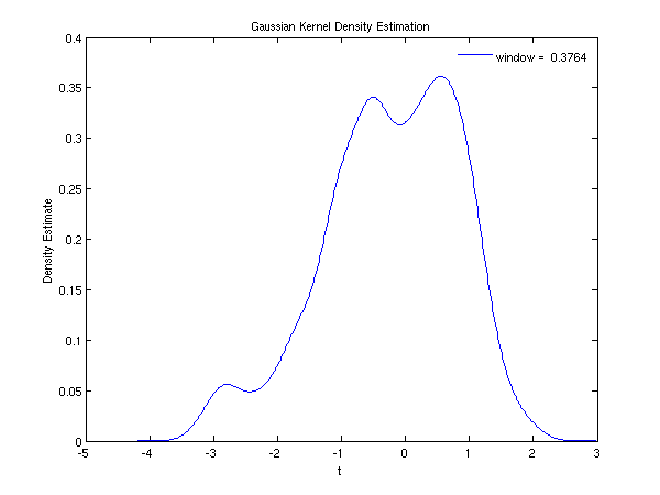
fig1 = figure;
plot(t,smooth);
title('Gaussian Kernel Density Estimation');
xlabel('t');
ylabel('Density Estimate');
wind_leg = sprintf('window = %7.4f',window);
legend(wind_leg);
legend('boxoff');

g10bb example results

Window Width Used =  3.7638e-01
Interval = (-4.1882e+00, 2.9822e+00)

First 20 output values:

    Time point      Density estimate
    ----------      ----------------
       -4.1811        3.8281e-06
       -4.1671        4.0305e-06
       -4.1531        4.4233e-06
       -4.1391        5.0212e-06
       -4.1251        5.8461e-06
       -4.1111        6.9279e-06
       -4.0971        8.3048e-06
       -4.0831        1.0025e-05
       -4.0691        1.2145e-05
       -4.0551        1.4736e-05
       -4.0411        1.7881e-05
       -4.0271        2.1677e-05
       -4.0131        2.6239e-05
       -3.9991        3.1700e-05
       -3.9851        3.8214e-05
       -3.9711        4.5960e-05
       -3.9571        5.5141e-05
       -3.9431        6.5990e-05
       -3.9291        7.8775e-05
       -3.9151        9.3796e-05

References

Jones M C and Lotwick H W (1984) Remark AS R50. A remark on algorithm AS 176. Kernel density estimation using the Fast Fourier Transform Appl. Statist. 33 120–122
Silverman B W (1982) Algorithm AS 176. Kernel density estimation using the fast Fourier transform Appl. Statist. 31 93–99
Silverman B W (1990) Density Estimation Chapman and Hall