PDF version (NAG web site
, 64-bit version, 64-bit version)
NAG Toolbox: nag_correg_quantile_linreg_easy (g02qf)
Purpose
nag_correg_quantile_linreg_easy (g02qf) performs a multiple linear quantile regression, returning the parameter estimates and associated confidence limits based on an assumption of Normal, independent, identically distributed errors.
nag_correg_quantile_linreg_easy (g02qf) is a simplified version of
nag_correg_quantile_linreg (g02qg).
Syntax
[
df,
b,
bl,
bu,
info,
ifail] = g02qf(
x,
y,
tau, 'n',
n, 'm',
m, 'ntau',
ntau)
[
df,
b,
bl,
bu,
info,
ifail] = nag_correg_quantile_linreg_easy(
x,
y,
tau, 'n',
n, 'm',
m, 'ntau',
ntau)
Description
Given a vector of
observed values,
, an
design matrix
, a column vector,
, of length
holding the
th row of
and a quantile
,
nag_correg_quantile_linreg_easy (g02qf) estimates the
-element vector
as the solution to
where
is the piecewise linear loss function
, and
is an indicator function taking the value
if
and
otherwise.
nag_correg_quantile_linreg_easy (g02qf) assumes Normal, independent, identically distributed (IID) errors and calculates the asymptotic covariance matrix from
where
is the sparsity function, which is estimated from the residuals,
(see
Koenker (2005)).
Given an estimate of the covariance matrix,
, lower,
, and upper,
, limits for a
confidence interval are calculated for each of the
parameters, via
where
is the
percentile of the Student's
distribution with
degrees of freedom, where
is the rank of the cross-product matrix
.
Further details of the algorithms used by
nag_correg_quantile_linreg_easy (g02qf) can be found in the documentation for
nag_correg_quantile_linreg (g02qg).
References
Koenker R (2005) Quantile Regression Econometric Society Monographs, Cambridge University Press, New York
Parameters
Compulsory Input Parameters
- 1:
– double array
-
, the design matrix, with the
th value for the th variate supplied in , for and .
- 2:
– double array
-
, the observations on the dependent variable.
- 3:
– double array
-
The vector of quantiles of interest. A separate model is fitted to each quantile.
Constraint:
where
is the
machine precision returned by
nag_machine_precision (x02aj), for
.
Optional Input Parameters
- 1:
– int64int32nag_int scalar
-
Default:
the dimension of the array
y and the first dimension of the array
x. (An error is raised if these dimensions are not equal.)
, the number of observations in the dataset.
Constraint:
.
- 2:
– int64int32nag_int scalar
-
Default:
the second dimension of the array
x.
, the number of variates in the model.
Constraint:
.
- 3:
– int64int32nag_int scalar
-
Default:
the dimension of the array
tau.
The number of quantiles of interest.
Constraint:
.
Output Parameters
- 1:
– double scalar
-
The degrees of freedom given by , where is the number of observations and is the rank of the cross-product matrix .
- 2:
– double array
-
, the estimates of the parameters of the regression model, with
containing the coefficient for the variable in column
of
x, estimated for
.
- 3:
– double array
-
, the lower limit of a confidence interval for , with holding the lower limit associated with .
- 4:
– double array
-
, the upper limit of a confidence interval for , with holding the upper limit associated with .
- 5:
– int64int32nag_int array
-
holds additional information concerning the model fitting and confidence limit calculations when
.
| Code | Warning |
| Model fitted and confidence limits calculated successfully. |
| The function did not converge whilst calculating the parameter estimates. The returned values are based on the estimate at the last iteration. |
| A singular matrix was encountered during the optimization. The model was not fitted for this value of . |
| The function did not converge whilst calculating the confidence limits. The returned limits are based on the estimate at the last iteration. |
| Confidence limits for this value of could not be calculated. The returned upper and lower limits are set to a large positive and large negative value respectively. |
It is possible for multiple warnings to be applicable to a single model. In these cases the value returned in
info is the sum of the corresponding individual nonzero warning codes.
- 6:
– int64int32nag_int scalar
unless the function detects an error (see
Error Indicators and Warnings).
Error Indicators and Warnings
Errors or warnings detected by the function:
-
-
Constraint: .
-
-
Constraint: .
-
-
Constraint: .
-
-
On entry is invalid.
-
-
A potential problem occurred whilst fitting the model(s).
Additional information has been returned in
info.
-
An unexpected error has been triggered by this routine. Please
contact
NAG.
-
Your licence key may have expired or may not have been installed correctly.
-
Dynamic memory allocation failed.
Accuracy
Not applicable.
Further Comments
Calling
nag_correg_quantile_linreg_easy (g02qf) is equivalent to calling
nag_correg_quantile_linreg (g02qg) with
- ,
- ,
-
,
- ,
- setting each element of isx to ,
- ,
- , and
- .
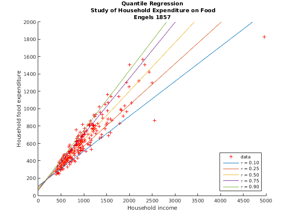
Example
A quantile regression model is fitted to Engels 1857 study of household expenditure on food. The model regresses the dependent variable, household food expenditure, against household income. An intercept is included in the model by augmenting the dataset with a column of ones.
Open in the MATLAB editor:
g02qf_example
function g02qf_example
fprintf('g02qf example results\n\n');
n = 235;
x = zeros(n,2);
x(:,1) = ones(n,1);
x(:,2) = ...
[ 420.1577 800.7990 643.3571 541.4117 1245.6964 2551.6615 901.1575 ...
1201.0002 1795.3226 639.0802 634.4002 1165.7734 750.8756 956.2315 ...
815.6212 945.7989 1148.6010 1264.2066 829.3979 1768.8236 1095.4056 ...
979.1648 2822.5330 447.4479 1309.8789 922.3548 1178.9742 1492.3987 ...
2293.1920 975.8023 502.8390 627.4726 1017.8522 616.7168 889.9809 ...
423.8798 790.9225 1162.2000 558.7767 555.8786 1197.0794 943.2487 ...
713.4412 530.7972 1348.3002 838.7561 1142.1526 2340.6174 535.0766 ...
1088.0039 587.1792 596.4408 484.6612 1540.9741 924.5619 1536.0201 ...
1115.8481 487.7583 678.8974 1044.6843 692.6397 671.8802 1389.7929 ...
997.8770 690.4683 2497.7860 506.9995 860.6948 1585.3809 654.1587 ...
873.3095 1862.0438 933.9193 894.4598 2008.8546 433.6813 1148.6470 ...
697.3099 587.5962 926.8762 571.2517 896.4746 839.0414 598.3465 ...
454.4782 829.4974 461.0977 584.9989 1264.0043 977.1107 800.7990 ...
1937.9771 883.9849 502.4369 698.8317 718.3594 713.5197 920.4199 ...
543.8971 906.0006 1897.5711 1587.3480 880.5969 891.6824 4957.8130 ...
796.8289 889.6784 969.6838 854.8791 1221.4818 419.9980 1167.3716 ...
544.5991 561.9990 523.8000 1031.4491 689.5988 670.7792 1462.9497 ...
1398.5203 377.0584 830.4353 820.8168 851.5430 975.0415 875.1716 ...
1121.0937 1337.9983 1392.4499 625.5179 867.6427 1256.3174 805.5377 ...
725.7459 1362.8590 558.5812 989.0056 1999.2552 884.4005 1525.0005 ...
1209.4730 1257.4989 672.1960 1125.0356 2051.1789 923.3977 1827.4010 ...
1466.3330 472.3215 1014.1540 730.0989 590.7601 880.3944 2432.3910 ...
831.7983 873.7375 940.9218 1139.4945 951.4432 1177.8547 507.5169 ...
473.0022 1222.5939 576.1972 601.0030 1519.5811 696.5991 713.9979 ...
687.6638 650.8180 829.2984 953.1192 949.5802 959.7953 953.1192 ...
497.1193 1212.9613 953.1192 570.1674 958.8743 939.0418 724.7306 ...
1129.4431 1283.4025 408.3399 1943.0419 1511.5789 638.6713 539.6388 ...
1342.5821 1225.7890 463.5990 511.7980 715.3701 562.6400 689.7988 ...
800.4708 736.7584 1532.3074 975.5974 1415.4461 1056.0808 1613.7565 ...
2208.7897 387.3195 608.5019 636.0009 387.3195 958.6634 759.4010 ...
410.9987 835.9426 1078.8382 499.7510 1024.8177 748.6413 832.7554 ...
1006.4353 987.6417 614.9986 726.0000 788.0961 887.4658 494.4174 ...
1020.0225 1595.1611 776.5958 1230.9235 1807.9520 415.4407 440.5174 ...
541.2006 581.3599 743.0772 1057.6767];
y = [ 255.8394 572.0807 459.8177 310.9587 907.3969 863.9199 485.6800 ...
811.5776 831.4407 402.9974 427.7975 534.7610 495.5608 649.9985 ...
392.0502 633.7978 860.6002 934.9752 630.7566 1143.4211 813.3081 ...
700.4409 2032.6792 263.7100 830.9586 590.6183 769.0838 815.3602 ...
1570.3911 630.5863 338.0014 483.4800 645.9874 412.3613 600.4804 ...
319.5584 520.0006 696.2021 348.4518 452.4015 774.7962 614.5068 ...
512.7201 390.5984 662.0096 658.8395 612.5619 1504.3708 392.5995 ...
708.7622 406.2180 443.5586 296.9192 692.1689 640.1164 1071.4627 ...
588.1371 333.8394 496.5976 511.2609 466.9583 503.3974 700.5600 ...
543.3969 357.6411 1301.1451 317.7198 430.3376 879.0660 424.3209 ...
624.6990 912.8851 518.9617 582.5413 1509.7812 338.0014 580.2215 ...
484.0605 419.6412 543.8807 399.6703 476.3200 588.6372 444.1001 ...
386.3602 627.9999 248.8101 423.2783 712.1012 527.8014 503.3572 ...
968.3949 500.6313 354.6389 482.5816 436.8107 497.3182 593.1694 ...
374.7990 588.5195 1033.5658 726.3921 654.5971 693.6795 1827.2000 ...
550.7274 693.6795 523.4911 528.3770 761.2791 334.9998 640.4813 ...
361.3981 473.2009 401.3204 628.4522 581.2029 435.9990 771.4486 ...
929.7540 276.5606 757.1187 591.1974 588.3488 821.5970 637.5483 ...
664.1978 1022.3202 674.9509 444.8602 679.4407 776.7589 462.8995 ...
538.7491 959.5170 377.7792 679.9981 1250.9643 553.1504 977.0033 ...
737.8201 810.8962 561.2015 810.6772 1067.9541 728.3997 983.0009 ...
1049.8788 372.3186 708.8968 522.7012 361.5210 633.1200 1424.8047 ...
620.8006 631.7982 517.9196 819.9964 608.6419 830.9586 360.8780 ...
300.9999 925.5795 395.7608 377.9984 1162.0024 442.0001 397.0015 ...
383.4580 404.0384 588.5195 621.1173 670.7993 681.7616 621.1173 ...
297.5702 807.3603 621.1173 353.4882 696.8011 548.6002 383.9376 ...
811.1962 745.2353 284.8008 1305.7201 837.8005 431.1000 442.0001 ...
795.3402 801.3518 353.6013 418.5976 448.4513 468.0008 508.7974 ...
577.9111 526.7573 883.2780 570.5210 890.2390 742.5276 865.3205 ...
1318.8033 242.3202 444.5578 331.0005 242.3202 680.4198 416.4015 ...
266.0010 576.2779 596.8406 408.4992 708.4787 429.0399 614.7588 ...
734.2356 619.6408 385.3184 433.0010 400.7990 515.6200 327.4188 ...
775.0209 1138.1620 485.5198 772.7611 993.9630 305.4390 306.5191 ...
299.1993 468.0008 522.6019 750.3202];
tau = [0.10; 0.25; 0.50; 0.75; 0.90];
[df, b, bl, bu, info, ifail] = g02qf( ...
x, y, tau);
t = '\tau';
fig1 = figure;
hold on;
plot(x(:,2),y,'+r');
tt{1} = 'data';
for l=1:numel(tau)
fprintf('\nQuantile: %6.3f\n\n', tau(l));
fprintf(' Lower Parameter Upper\n');
fprintf(' Limit Estimate Limit\n');
for j=1:2
fprintf('%3d %7.3f %7.3f %7.3f\n', j, bl(j,l), b(j,l), bu(j,l));
end
fprintf('\n');
plot([0 (2000-b(1,l))/b(2,l)],[b(1,l) 2000]);
tt{l+1} = sprintf('%s = %4.2f',t,tau(l));
end
legend(tt,'Location','SouthEast')
xlabel('Household income');
ylabel('Household food expenditure');
title({'Quantile Regression', ...
' Study of Household Expenditure on Food', ...
'Engels 1857'});
axis([0 5000 0 2000]);
hold off;
g02qf example results


Quantile:  0.100

        Lower   Parameter   Upper
        Limit   Estimate    Limit
  1    74.946   110.142   145.337
  2     0.370     0.402     0.433


Quantile:  0.250

        Lower   Parameter   Upper
        Limit   Estimate    Limit
  1    64.232    95.483   126.735
  2     0.446     0.474     0.502


Quantile:  0.500

        Lower   Parameter   Upper
        Limit   Estimate    Limit
  1    55.399    81.482   107.566
  2     0.537     0.560     0.584


Quantile:  0.750

        Lower   Parameter   Upper
        Limit   Estimate    Limit
  1    41.372    62.396    83.421
  2     0.625     0.644     0.663


Quantile:  0.900

        Lower   Parameter   Upper
        Limit   Estimate    Limit
  1    26.829    67.351   107.873
  2     0.650     0.686     0.723
PDF version (NAG web site
, 64-bit version, 64-bit version)
© The Numerical Algorithms Group Ltd, Oxford, UK. 2009–2015