hide long namesshow long names
hide short namesshow short names
Integer type:  int32  int64  nag_int  show int32  show int32  show int64  show int64  show nag_int  show nag_int

PDF version (NAG web site, 64-bit version, 64-bit version)
Chapter Contents
Chapter Introduction
NAG Toolbox

NAG Toolbox: nag_ode_bvp_coll_nlin_diag (d02tz)

 Contents

    1  Purpose
    2  Syntax
    7  Accuracy
    9  Example

Purpose

nag_ode_bvp_coll_nlin_diag (d02tz) returns information about the solution of a general two-point boundary value problem computed by nag_ode_bvp_coll_nlin_solve (d02tl).

Syntax

[nmesh, mesh, ipmesh, ermx, iermx, ijermx, ifail] = d02tz(mxmesh, rcomm, icomm)
[nmesh, mesh, ipmesh, ermx, iermx, ijermx, ifail] = nag_ode_bvp_coll_nlin_diag(mxmesh, rcomm, icomm)

Description

nag_ode_bvp_coll_nlin_diag (d02tz) and its associated functions (nag_ode_bvp_coll_nlin_solve (d02tl), nag_ode_bvp_coll_nlin_setup (d02tv), nag_ode_bvp_coll_nlin_contin (d02tx) and nag_ode_bvp_coll_nlin_interp (d02ty)) solve the two-point boundary value problem for a nonlinear mixed order system of ordinary differential equations
y1m1 x = f1 x,y1,y11,,y1m1-1,y2,,ynmn-1 y2m2 x = f2 x,y1,y11,,y1m1-1,y2,,ynmn-1 ynmn x = fn x,y1,y11,,y1m1-1,y2,,ynmn-1  
over an interval a,b subject to p (>0) nonlinear boundary conditions at a and q (>0) nonlinear boundary conditions at b, where p+q = i=1 n mi . Note that yi m x is the mth derivative of the ith solution component. Hence yi 0 x=yix. The left boundary conditions at a are defined as
gizya=0,  i=1,2,,p,  
and the right boundary conditions at b as
g-jzyb=0,  j=1,2,,q,  
where y=y1,y2,,yn and
zyx = y1x, y11 x ,, y1m1-1 x ,y2x,, ynmn-1 x .  
First, nag_ode_bvp_coll_nlin_setup (d02tv) must be called to specify the initial mesh, error requirements and other details. Then, nag_ode_bvp_coll_nlin_solve (d02tl) can be used to solve the boundary value problem. After successful computation, nag_ode_bvp_coll_nlin_diag (d02tz) can be used to ascertain details about the final mesh. nag_ode_bvp_coll_nlin_interp (d02ty) can be used to compute the approximate solution anywhere on the interval a,b using interpolation.
The functions are based on modified versions of the codes COLSYS and COLNEW (see Ascher et al. (1979) and Ascher and Bader (1987)). A comprehensive treatment of the numerical solution of boundary value problems can be found in Ascher et al. (1988) and Keller (1992).

References

Ascher U M and Bader G (1987) A new basis implementation for a mixed order boundary value ODE solver SIAM J. Sci. Stat. Comput. 8 483–500
Ascher U M, Christiansen J and Russell R D (1979) A collocation solver for mixed order systems of boundary value problems Math. Comput. 33 659–679
Ascher U M, Mattheij R M M and Russell R D (1988) Numerical Solution of Boundary Value Problems for Ordinary Differential Equations Prentice–Hall
Cole J D (1968) Perturbation Methods in Applied Mathematics Blaisdell, Waltham, Mass.
Keller H B (1992) Numerical Methods for Two-point Boundary-value Problems Dover, New York

Parameters

Compulsory Input Parameters

1:     mxmesh int64int32nag_int scalar
The maximum number of points allowed in the mesh.
Constraint: this must be identical to the value supplied for the argument mxmesh in the prior call to nag_ode_bvp_coll_nlin_setup (d02tv).
2:     rcomm* – double array
Note: the dimension of this array is dictated by the requirements of associated functions that must have been previously called. This array must be the same array passed as argument rcomm in the previous call to nag_ode_bvp_coll_nlin_solve (d02tl).
This must be the same array as supplied to nag_ode_bvp_coll_nlin_solve (d02tl) and must remain unchanged between calls.
3:     icomm* int64int32nag_int array
Note: the dimension of this array is dictated by the requirements of associated functions that must have been previously called. This array must be the same array passed as argument icomm in the previous call to nag_ode_bvp_coll_nlin_solve (d02tl).
This must be the same array as supplied to nag_ode_bvp_coll_nlin_solve (d02tl) and must remain unchanged between calls.

Optional Input Parameters

None.

Output Parameters

1:     nmesh int64int32nag_int scalar
The number of points in the mesh last used by nag_ode_bvp_coll_nlin_solve (d02tl).
2:     meshmxmesh – double array
meshi contains the ith point of the mesh last used by nag_ode_bvp_coll_nlin_solve (d02tl), for i=1,2,,nmesh. mesh1 will contain a and meshnmesh will contain b. The remaining elements of mesh are not initialized.
3:     ipmeshmxmesh int64int32nag_int array
ipmeshi specifies the nature of the point meshi, for i=1,2,,nmesh, in the final mesh computed by nag_ode_bvp_coll_nlin_solve (d02tl).
ipmeshi=1
Indicates that the ith point is a fixed point and was used by the solver before an extrapolation-like error test.
ipmeshi=2
Indicates that the ith point was used by the solver before an extrapolation-like error test.
ipmeshi=3
Indicates that the ith point was used by the solver only as part of an extrapolation-like error test.
The remaining elements of ipmesh are initialized to -1.
See Further Comments for advice on how these values may be used in conjunction with a continuation process.
4:     ermx – double scalar
An estimate of the maximum error in the solution computed by nag_ode_bvp_coll_nlin_solve (d02tl), that is
ermx=maxyi-vi 1.0+vi  
where vi is the approximate solution for the ith solution component. If nag_ode_bvp_coll_nlin_solve (d02tl) returned successfully with ifail=0, then ermx will be less than tolsijermx where tols contains the error requirements as specified in Description and Arguments in nag_ode_bvp_coll_nlin_setup (d02tv).
If nag_ode_bvp_coll_nlin_solve (d02tl) returned with ifail=5, then ermx will be greater than tolsijermx.
If nag_ode_bvp_coll_nlin_solve (d02tl) returned any other value for ifail then an error estimate is not available and ermx is initialized to 0.0.
5:     iermx int64int32nag_int scalar
Indicates the mesh sub-interval where the value of ermx has been computed, that is mesh iermx ,mesh iermx + 1 .
If an estimate of the error is not available then iermx is initialized to 0.
6:     ijermx int64int32nag_int scalar
Indicates the component i (=ijermx) of the solution for which ermx has been computed, that is the approximation of yi on meshiermx,meshiermx+1 is estimated to have the largest error of all components yi over mesh sub-intervals defined by mesh.
If an estimate of the error is not available then ijermx is initialized to 0.
7:     ifail int64int32nag_int scalar
ifail=0 unless the function detects an error (see Error Indicators and Warnings).

Error Indicators and Warnings

Note: nag_ode_bvp_coll_nlin_diag (d02tz) may return useful information for one or more of the following detected errors or warnings.
Errors or warnings detected by the function:
   ifail=1
On entry, an illegal value for mxmesh was specified, or an invalid call to nag_ode_bvp_coll_nlin_diag (d02tz) was made, for example without a previous call to the solver function nag_ode_bvp_coll_nlin_solve (d02tl).
   ifail=2
The solver function nag_ode_bvp_coll_nlin_solve (d02tl) did not converge to a solution or did not satisfy the error requirements. The last mesh computed by nag_ode_bvp_coll_nlin_solve (d02tl) has been returned by nag_ode_bvp_coll_nlin_diag (d02tz). This mesh should be treated with extreme caution as nothing can be said regarding its quality or suitability for any subsequent computation.
   ifail=-99
An unexpected error has been triggered by this routine. Please contact NAG.
   ifail=-399
Your licence key may have expired or may not have been installed correctly.
   ifail=-999
Dynamic memory allocation failed.

Accuracy

Not applicable.

Further Comments

Note that:
If nag_ode_bvp_coll_nlin_diag (d02tz) returns ifail=0, then examination of the mesh may provide assistance in determining a suitable starting mesh for nag_ode_bvp_coll_nlin_setup (d02tv) in any subsequent attempts to solve similar problems.
If the problem being treated by nag_ode_bvp_coll_nlin_solve (d02tl) is one of a series of related problems (for example, as part of a continuation process), then the values of ipmesh and mesh may be suitable as input arguments to nag_ode_bvp_coll_nlin_contin (d02tx). Using the mesh points not involved in the extrapolation error test is usually appropriate. ipmesh and mesh should be passed unchanged to nag_ode_bvp_coll_nlin_contin (d02tx) but nmesh should be replaced by nmesh+1/2.
If nag_ode_bvp_coll_nlin_diag (d02tz) returns ifail=2, nothing can be said regarding the quality of the mesh returned. However, it may be a useful starting mesh for nag_ode_bvp_coll_nlin_setup (d02tv) in any subsequent attempts to solve the same problem.
If nag_ode_bvp_coll_nlin_solve (d02tl) returns ifail=5, this corresponds to the solver requiring more than mxmesh mesh points to satisfy the error requirements. If mxmesh can be increased and the preceding call to nag_ode_bvp_coll_nlin_solve (d02tl) was not part, or was the first part, of a continuation process then the values in mesh may provide a suitable mesh with which to initialize a subsequent attempt to solve the same problem. If it is not possible to provide more mesh points then relaxing the error requirements by setting tolsijermx to ermx might lead to a successful solution. It may be necessary to reset the other components of tols. Note that resetting the tolerances can lead to a different sequence of meshes being computed and hence to a different solution being computed.

Example

The following example is used to illustrate the use of fixed mesh points, simple continuation and numerical approximation of a Jacobian. See also nag_ode_bvp_coll_nlin_solve (d02tl), nag_ode_bvp_coll_nlin_setup (d02tv), nag_ode_bvp_coll_nlin_contin (d02tx) and nag_ode_bvp_coll_nlin_interp (d02ty), for the illustration of other facilities.
Consider the Lagerstrom–Cole equation
y=y-yy/ε  
with the boundary conditions
y0=αy1=β, (1)
where ε is small and positive. The nature of the solution depends markedly on the values of α,β. See Cole (1968).
We choose α=-13,β=13  for which the solution is known to have corner layers at x=13,23 . We choose an initial mesh of seven points 0.0,0.15,0.3,0.5,0.7,0.85,1.0 and ensure that the points x=0.3,0.7 near the corner layers are fixed, that is the corresponding elements of the array ipmesh are set to 1. First we compute the solution for ε=1.0e−4 using in guess the initial approximation yx=α+β-αx which satisfies the boundary conditions. Then we use simple continuation to compute the solution for ε=1.0e−5. We use the suggested values for nmesh, ipmesh and mesh in the call to nag_ode_bvp_coll_nlin_contin (d02tx) prior to the continuation call, that is only every second point of the preceding mesh is used and the fixed mesh points are retained.
Although the analytic Jacobian for this system is easy to evaluate, for illustration the procedure fjac uses central differences and calls to ffun to compute a numerical approximation to the Jacobian.
function d02tz_example


fprintf('d02tz example results\n\n');

global alpha beta eps; % For communication with local functions

% Initialize variables and arrays.
neq  = int64(1);
nlbc = int64(1);
nrbc = int64(1);
ncol = int64(5);
mmax = int64(2);
m    = int64([2]);
tols = [1.0e-05];

% Set values for problem-specific physical parameters.
alpha = -1/3;
beta  =  1/3;
eps   = 1e-3;

% Set up the mesh.
nmesh  = int64(7);
mxmesh = int64(50);

% Set location of mesh points, and specify which are fixed.
mesh =   zeros(mxmesh, 1);
ipmesh = zeros(mxmesh, 1, 'int64');
mesh(1:nmesh) =  [0.0; 0.15; 0.3; 0.5; 0.7; 0.85; 1.0];
ipmesh(1:2:nmesh) = 1;
ipmesh(2:2:nmesh) = 2;

% Prepare to store results for plotting.
xarray = zeros(1,1);
yarray = zeros(1,2);

% d02tv is a setup routine to be called prior to d02tk.
[work, iwork, ifail] = d02tv( ...
                              m, nlbc, nrbc, ncol, tols, nmesh, mesh, ipmesh);
ncont = 2;

% We run through the calculation ncont times with different parameter sets.
for jcont = 1:ncont

  eps = 0.1*eps;
  fprintf('\n Tolerance = %8.1e, eps = %10.3e\n\n', tols(1), eps);

  % Call d02tk to solve BVP for this set of parameters.
  [work, iwork, ifail] = d02tk( ...
                                @ffun, @fjac, @gafun, @gbfun, @gajac, ...
                                @gbjac, @guess, work, iwork);
  % Call d02tz to extract mesh from solution.
  [nmesh, mesh, ipmesh, ermx, iermx, ijermx, ifail] = ...
  d02tz( ...
         mxmesh, work, iwork);

    % Output mesh results.
  fprintf(' Used a mesh of %d points\n', nmesh);
  fprintf(' Maximum error = %10.2e in interval %d for component %d\n\n',...
          ermx, iermx, ijermx);

  % Output solution, and store it for plotting.
  fprintf(' Solution and derivative at every second point:\n');
  fprintf('      x        u          u''\n');
  for imesh = 1:nmesh

    % Call d02ty to perform interpolation on the solution.
    [y, work, ifail] = d02ty( ...
                              mesh(imesh), neq, mmax, work, iwork);
    if mod(imesh, 2) ~= 0
      fprintf(' %8.4f   %8.5f   %8.5f\n', mesh(imesh), y(1,1), y(1,2));
    end
    xarray(imesh) = mesh(imesh);
    yarray(imesh, :) = y(1, :);
  end

  % Plot results for this parameter set.
  if jcont==1
    fig1 = figure;
  else
    fig2 = figure;
  end
  display_plot(xarray, yarray, eps)
  
  % Select mesh for next calculation.
  if jcont < ncont
    nmesh = (nmesh+1)/2;

    % d02tx allows the current solution to be used as an initial
    % approximation to the solution of a related problem.
    [work, iwork, ifail] = d02tx( ...
                                  nmesh, mesh, ipmesh, work, iwork);
  end
end


function [f] = ffun(x, y, neq, m)
  % Evaluate derivative functions (rhs of system of ODEs).

  global eps
  f = zeros(neq, 1);
  f(1) = (y(1,1) - y(1,1)*y(1,2))/eps;
  
function [dfdy] = fjac(x, y, neq, m)
  % Evaluate Jacobians (partial derivatives of f).

  dfdy = zeros(neq, neq, 1);

  machep = x02aj;
  fac = sqrt(machep);
  for i = 1:neq
    yp(i,1:m(i)) = y(i,1:m(i));
  end

  for i = 1:neq
    for j = 1:m(i)
      ptrb = max(100*machep, fac*abs(y(i,j)));
      yp(i,j) = y(i,j) + ptrb;
      f1 = ffun(x, yp, neq, m);
      yp(i,j) = y(i,j) - ptrb;
      f2 = ffun(x, yp, neq, m);
      dfdy(:,i,j) = 0.5*(f1- f2)/ptrb;
      yp(i,j) = y(i,j);
    end
  end

function [ga] = gafun(ya, neq, m, nlbc)
  % Evaluate boundary conditions at left-hand end of range.

  global alpha beta
  ga = zeros(nlbc, 1);
  ga(1) = ya(1,1) - alpha;

function [dgady] = gajac(ya, neq, m, nlbc)
  % Evaluate Jacobians (partial derivatives of ga).

  dgady = zeros(nlbc, neq, 2);
  dgady(1,1,1) = 1;

function [gb] = gbfun(yb, neq, m, nrbc)
  % Evaluate boundary conditions at right-hand end of range.

  global alpha beta
  gb = zeros(nrbc, 1);
  gb(1) = yb(1,1) - beta;

function [dgbdy] = gbjac(yb, neq, m, nrbc)
  % Evaluate Jacobians (partial derivatives of gb).

  dgbdy = zeros(nrbc, neq, 2);
  dgbdy(1,1,1) = 1;

function [y, dym] = guess(x, neq, m)
  % Evaluate initial approximations to solution components and derivatives.

  global alpha beta
  y = zeros(neq, 2);
  dym = zeros(neq, 1);
  y(1,1) = alpha + (beta - alpha)*x;
  y(1,2) = beta - alpha;
  dym(1) = 0;

function display_plot(x, y, eps)
  % Plot the results.
  [haxes, hline1, hline2] = plotyy(x, y(:,1), x, y(:,2));
  % Set the axis limits and the tick specifications to beautify the plot.
  set(haxes(1), 'YLim', [-0.5 0.5]);
  set(haxes(1), 'YMinorTick', 'on');
  set(haxes(1), 'YTick', [-0.5 -0.25 0 0.25 0.5]);
  set(haxes(2), 'YLim', [0 2]);
  set(haxes(2), 'YTick', [0 0.25 0.5 0.75 1.0 1.25 1.5 1.75 2]);
  set(haxes(2), 'YMinorTick', 'on');
  for iaxis = 1:2
    % These properties must be the same for both sets of axes.
    set(haxes(iaxis), 'XLim', [0 1]);
  end
  set(gca, 'box', 'off')
  % Add title.
  title('Largerstrom-Cole Equation (-1/3, 1/3)');
  text(0.4,0.4,['eps = ', num2str(eps)]);
  % Label the axes.
  xlabel('x');
  ylabel(haxes(1), 'Solution');
  ylabel(haxes(2), 'Derivative');
  % Add a legend.
  legend('solution','derivative','Location','Best');
  % Set some features of the three lines.
  set(hline1, 'Linewidth', 0.25, 'Marker', '+', 'LineStyle', '-');
  set(hline2, 'Linewidth', 0.25, 'Marker', 'x', 'LineStyle', '--');
d02tz example results


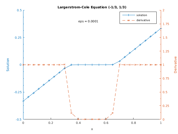
 Tolerance =  1.0e-05, eps =  1.000e-04

 Used a mesh of 25 points
 Maximum error =   2.15e-06 in interval 16 for component 1

 Solution and derivative at every second point:
      x        u          u'
   0.0000   -0.33333    1.00000
   0.0750   -0.25833    1.00000
   0.1500   -0.18333    1.00000
   0.2250   -0.10833    1.00002
   0.3000   -0.03332    1.00372
   0.4000   -0.00001    0.00084
   0.5000   -0.00000    0.00000
   0.6000    0.00001    0.00084
   0.7000    0.03332    1.00372
   0.7750    0.10833    1.00002
   0.8500    0.18333    1.00000
   0.9250    0.25833    1.00000
   1.0000    0.33333    1.00000

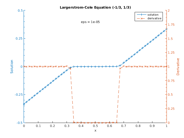
 Tolerance =  1.0e-05, eps =  1.000e-05

 Used a mesh of 49 points
 Maximum error =   2.11e-06 in interval 32 for component 1

 Solution and derivative at every second point:
      x        u          u'
   0.0000   -0.33333    1.00014
   0.0375   -0.29583    1.00018
   0.0750   -0.25833    1.00022
   0.1125   -0.22083    1.00029
   0.1500   -0.18333    1.00040
   0.1875   -0.14583    1.00059
   0.2250   -0.10833    1.00098
   0.2625   -0.07083    1.00202
   0.3000   -0.03333    1.00745
   0.3500   -0.00001    0.00354
   0.4000   -0.00000    0.00000
   0.4500   -0.00000    0.00000
   0.5000    0.00000   -0.00000
   0.5500    0.00000    0.00000
   0.6000    0.00000    0.00000
   0.6500    0.00001    0.00354
   0.7000    0.03333    1.00745
   0.7375    0.07083    1.00202
   0.7750    0.10833    1.00098
   0.8125    0.14583    1.00059
   0.8500    0.18333    1.00040
   0.8875    0.22083    1.00029
   0.9250    0.25833    1.00022
   0.9625    0.29583    1.00018
   1.0000    0.33333    1.00014
d02tz_fig1.png
d02tz_fig2.png

PDF version (NAG web site, 64-bit version, 64-bit version)
Chapter Contents
Chapter Introduction
NAG Toolbox

© The Numerical Algorithms Group Ltd, Oxford, UK. 2009–2015