e04wd is designed to minimize an arbitrary smooth function subject to constraints (which may include simple bounds on the variables, linear constraints and smooth nonlinear constraints) using a sequential quadratic programming (SQP) method. As many first derivatives as possible should be supplied by you; any unspecified derivatives are approximated by finite differences. It is not intended for large sparse problems.

e04wd may also be used for unconstrained, bound-constrained and linearly constrained optimization.

e04wd uses forward communication for evaluating the objective function, the nonlinear constraint functions, and any of their derivatives.

The initialization method (E04WCF not in this release) must have been called before to calling e04wd.

Syntax

C#
public static void e04wd( int n, int nclin, int ncnln, double[,] a, double[] bl, double[] bu, E04..::..E04WD_CONFUN confun, E04..::..E04WD_OBJFUN objfun, out int majits, int[] istate, double[] ccon, double[,] cjac, double[] clamda, out double objf, double[] grad, double[,] h, double[] x, E04..::..e04wdOptions options, out int ifail )

public static void e04wd(
	int n,
	int nclin,
	int ncnln,
	double[,] a,
	double[] bl,
	double[] bu,
	E04..::..E04WD_CONFUN confun,
	E04..::..E04WD_OBJFUN objfun,
	out int majits,
	int[] istate,
	double[] ccon,
	double[,] cjac,
	double[] clamda,
	out double objf,
	double[] grad,
	double[,] h,
	double[] x,
	E04..::..e04wdOptions options,
	out int ifail
)

Visual Basic
Public Shared Sub e04wd ( _ n As Integer, _ nclin As Integer, _ ncnln As Integer, _ a As Double(,), _ bl As Double(), _ bu As Double(), _ confun As E04..::..E04WD_CONFUN, _ objfun As E04..::..E04WD_OBJFUN, _ <OutAttribute> ByRef majits As Integer, _ istate As Integer(), _ ccon As Double(), _ cjac As Double(,), _ clamda As Double(), _ <OutAttribute> ByRef objf As Double, _ grad As Double(), _ h As Double(,), _ x As Double(), _ options As E04..::..e04wdOptions, _ <OutAttribute> ByRef ifail As Integer _ )

Visual Basic

Public Shared Sub e04wd ( _
	n As Integer, _
	nclin As Integer, _
	ncnln As Integer, _
	a As Double(,), _
	bl As Double(), _
	bu As Double(), _
	confun As E04..::..E04WD_CONFUN, _
	objfun As E04..::..E04WD_OBJFUN, _
	<OutAttribute> ByRef majits As Integer, _
	istate As Integer(), _
	ccon As Double(), _
	cjac As Double(,), _
	clamda As Double(), _
	<OutAttribute> ByRef objf As Double, _
	grad As Double(), _
	h As Double(,), _
	x As Double(), _
	options As E04..::..e04wdOptions, _
	<OutAttribute> ByRef ifail As Integer _
)

Visual C++
public: static void e04wd( int n, int nclin, int ncnln, array<double,2>^ a, array<double>^ bl, array<double>^ bu, E04..::..E04WD_CONFUN^ confun, E04..::..E04WD_OBJFUN^ objfun, [OutAttribute] int% majits, array<int>^ istate, array<double>^ ccon, array<double,2>^ cjac, array<double>^ clamda, [OutAttribute] double% objf, array<double>^ grad, array<double,2>^ h, array<double>^ x, E04..::..e04wdOptions^ options, [OutAttribute] int% ifail )

Visual C++

public:
static void e04wd(
	int n, 
	int nclin, 
	int ncnln, 
	array<double,2>^ a, 
	array<double>^ bl, 
	array<double>^ bu, 
	E04..::..E04WD_CONFUN^ confun, 
	E04..::..E04WD_OBJFUN^ objfun, 
	[OutAttribute] int% majits, 
	array<int>^ istate, 
	array<double>^ ccon, 
	array<double,2>^ cjac, 
	array<double>^ clamda, 
	[OutAttribute] double% objf, 
	array<double>^ grad, 
	array<double,2>^ h, 
	array<double>^ x, 
	E04..::..e04wdOptions^ options, 
	[OutAttribute] int% ifail
)

F#
static member e04wd : n : int * nclin : int * ncnln : int * a : float[,] * bl : float[] * bu : float[] * confun : E04..::..E04WD_CONFUN * objfun : E04..::..E04WD_OBJFUN * majits : int byref * istate : int[] * ccon : float[] * cjac : float[,] * clamda : float[] * objf : float byref * grad : float[] * h : float[,] * x : float[] * options : E04..::..e04wdOptions * ifail : int byref -> unit

static member e04wd : 
        n : int * 
        nclin : int * 
        ncnln : int * 
        a : float[,] * 
        bl : float[] * 
        bu : float[] * 
        confun : E04..::..E04WD_CONFUN * 
        objfun : E04..::..E04WD_OBJFUN * 
        majits : int byref * 
        istate : int[] * 
        ccon : float[] * 
        cjac : float[,] * 
        clamda : float[] * 
        objf : float byref * 
        grad : float[] * 
        h : float[,] * 
        x : float[] * 
        options : E04..::..e04wdOptions * 
        ifail : int byref -> unit

Parameters

n: Type: System..::..Int32
On entry: $n$ , the number of variables.

Constraint: $n > 0$ .

nclin: Type: System..::..Int32
On entry: $n_{L}$ , the number of general linear constraints.

Constraint: $nclin \geq 0$ .

ncnln: Type: System..::..Int32
On entry: $n_{N}$ , the number of nonlinear constraints.

Constraint: $ncnln \geq 0$ .

a: Type: array<System..::..Double,2>[,](,)[,][,]
An array of size [dim1, dim2]
Note: dim1 must satisfy the constraint: $dim1 \geq \max (1, nclin)$
Note: the second dimension of the array a must be at least $n$ if $nclin > 0$ , and at least $1$ otherwise.
On entry: the $i$ th row of a contains the $i$ th row of the matrix $A_{L}$ of general linear constraints in (1). That is, the $i$ th row contains the coefficients of the $i$ th general linear constraint, for $i = 1, 2, \dots, nclin$ .
If $nclin = 0$ , the array a is not referenced.

bl

Type: array<System..::..Double>[]()[][]

An array of size [

n + nclin + ncnln

]

On entry: bl must contain the lower bounds and bu the upper bounds for all the constraints, in the following order. The first

n

elements of each array must contain the bounds on the variables, the next

n_{L}

elements the bounds for the general linear constraints (if any) and the next

n_{N}

elements the bounds for the general nonlinear constraints (if any). To specify a nonexistent lower bound (i.e.,

l_{j} = - \infty

), set

bl [j - 1] \leq - bigbnd

, and to specify a nonexistent upper bound (i.e.,

u_{j} = + \infty

), set

bu [j - 1] \geq bigbnd

; where

bigbnd

is the optional parameter Infinite Bound Size. To specify the

j

th constraint as an equality, set

bl [j - 1] = bu [j - 1] = β

, say, where

|β| < bigbnd

Constraints:

$bl [j - 1] \leq bu [j - 1]$ , for $j = 1, 2, \dots, n + nclin + ncnln$ ;
if $bl [j - 1] = bu [j - 1] = β$ , $|β| < bigbnd$ .

bu

Type: array<System..::..Double>[]()[][]

An array of size [

n + nclin + ncnln

]

On entry: bl must contain the lower bounds and bu the upper bounds for all the constraints, in the following order. The first

n

elements of each array must contain the bounds on the variables, the next

n_{L}

elements the bounds for the general linear constraints (if any) and the next

n_{N}

elements the bounds for the general nonlinear constraints (if any). To specify a nonexistent lower bound (i.e.,

l_{j} = - \infty

), set

bl [j - 1] \leq - bigbnd

, and to specify a nonexistent upper bound (i.e.,

u_{j} = + \infty

), set

bu [j - 1] \geq bigbnd

; where

bigbnd

is the optional parameter Infinite Bound Size. To specify the

j

th constraint as an equality, set

bl [j - 1] = bu [j - 1] = β

, say, where

|β| < bigbnd

Constraints:

$bl [j - 1] \leq bu [j - 1]$ , for $j = 1, 2, \dots, n + nclin + ncnln$ ;
if $bl [j - 1] = bu [j - 1] = β$ , $|β| < bigbnd$ .

confun: Type: NagLibrary..::..E04..::..E04WD_CONFUN
confun must calculate the vector $c (x)$ of nonlinear constraint functions and (optionally) its Jacobian, $\frac{\partial c}{\partial x}$ , for a specified $n$ -vector $x$ . If there are no nonlinear constraints (i.e., $ncnln = 0$ ), e04wd will never call confun, so it may be the dummy method E04WDP. (E04WDP is included in the NAG Library). If there are nonlinear constraints, the first call to confun will occur before the first call to objfun.
If all constraint gradients (Jacobian elements) are known (i.e., $Derivative Level = 2$ or $3$ ), any constant elements may be assigned to cjac once only at the start of the optimization. An element of cjac that is not subsequently assigned in confun will retain its initial value throughout. Constant elements may be loaded in cjac during the first call to confun (signalled by the value of $nstate = 1$ ). The ability to preload constants is useful when many Jacobian elements are identically zero, in which case cjac may be initialized to zero and nonzero elements may be reset by confun.
It must be emphasized that, if $Derivative Level < 2$ , unassigned elements of cjac are not treated as constant; they are estimated by finite differences, at nontrivial expense.
A delegate of type E04WD_CONFUN.
confun should be tested separately before being used in conjunction with e04wd. See also the description of the optional parameter Verify Level.

objfun: Type: NagLibrary..::..E04..::..E04WD_OBJFUN
objfun must calculate the objective function $F (x)$ and (optionally) its gradient $g (x) = \frac{\partial F}{\partial x}$ for a specified $n$ -vector $x$ .
A delegate of type E04WD_OBJFUN.
objfun should be tested separately before being used in conjunction with e04wd. See also the description of the optional parameter Verify Level.

majits: Type: System..::..Int32%
On exit: the number of major iterations performed.

istate

Type: array<System..::..Int32>[]()[][]

An array of size [

n + nclin + ncnln

]

On entry: is an integer array that need not be initialized if e04wd is called with the Cold Start option (the default).

If optional parameter Warm Start has been chosen, every element of istate must be set. If e04wd has just been called on a problem with the same dimensions, istate already contains valid values. Otherwise,

istate [j - 1]

should indicate whether either of the constraints

r_{j} (x) \geq l_{j}

r_{j} (x) \leq u_{j}

is expected to be active at a solution of (1).

The ordering of istate is the same as for bl, bu and

r (x)

, i.e., the first n components of istate refer to the upper and lower bounds on the variables, the next nclin refer to the bounds on

A_{L} x

, and the last ncnln refer to the bounds on

c (x)

. Possible values of

istate [i - 1]

follow:

$0$	Neither $r_{j} (x) \geq l_{j}$ nor $r_{j} (x) \leq u_{j}$ is expected to be active.
$1$	$r_{j} (x) \geq l_{j}$ is expected to be active.
$2$	$r_{j} (x) \leq u_{j}$ is expected to be active.
$3$	This may be used if $l_{j} = u_{j}$ . Normally an equality constraint $r_{j} (x) = l_{j} = u_{j}$ is active at a solution.

The values

1

2

3

all have the same effect when

bl [j - 1] = bu [j - 1]

. If necessary, e04wd will override your specification of istate, so that a poor choice will not cause the algorithm to fail.

On exit: describes the status of the constraints

l \leq r (x) \leq u

. For the

j

th lower or upper bound,

j = 1, 2, \dots, n + nclin + ncnln

, the possible values of

istate [j - 1]

are as follows (see Figure 1).

δ

is the appropriate feasibility tolerance.

$- 2$	(Region 1) The lower bound is violated by more than $δ$ .
$- 1$	(Region 5) The upper bound is violated by more than $δ$ .
$0$	(Region 3) Both bounds are satisfied by more than $δ$ .
$1$	(Region 2) The lower bound is active (to within $δ$ ).
$2$	(Region 4) The upper bound is active (to within $δ$ ).
$3$	( $Region 2 = Region 4$ ) The bounds are equal and the equality constraint is satisfied (to within $δ$ ).

These values of istate are labelled in the printed solution according to Table 1.

Region	$1$	$2$	$3$	$4$	$5$	$2 \equiv 4$
$istate [j - 1]$	$- 2$	$1$	$0$	$2$	$- 1$	$3$
Printed solution	--	LL	FR	UL	++	EQ

Table 1
Labels used in the printed solution for the regions in Figure 1

ccon: Type: array<System..::..Double>[]()[][]
An array of size [ $\max (1, ncnln)$ ]
On entry: ccon need not be initialized if the (default) optional parameter Cold Start is used.
For a Warm Start, and if $ncnln > 0$ , ccon contains values of the nonlinear constraint functions $c_{i}$ , for $i = 1, 2, \dots, ncnln$ , calculated in a previous call to e04wd.

On exit: if $ncnln > 0$ , $ccon [i - 1]$ contains the value of the $i$ th nonlinear constraint function $c_{i}$ at the final iterate, for $i = 1, 2, \dots, ncnln$ .
If $ncnln = 0$ , the array ccon is not referenced.

cjac: Type: array<System..::..Double,2>[,](,)[,][,]
An array of size [dim1, dim2]
Note: dim1 must satisfy the constraint: $dim1 \geq \max (1, ncnln)$
Note: the second dimension of the array cjac must be at least $n$ if $ncnln > 0$ , and at least $1$ otherwise.
On entry: in general, cjac need not be initialized before the call to e04wd. However, if $Derivative Level = 2$ or $3$ , any constant elements of cjac may be initialized. Such elements need not be reassigned on subsequent calls to confun.
On exit: if $ncnln > 0$ , cjac contains the Jacobian matrix of the nonlinear constraint functions at the final iterate, i.e., $cjac [i - 1, j - 1]$ contains the partial derivative of the $i$ th constraint function with respect to the $j$ th variable, for $i = 1, 2, \dots, ncnln$ and $j = 1, 2, \dots, n$ . (See the discussion of parameter cjac under confun.)
If $ncnln = 0$ , the array cjac is not referenced.

clamda: Type: array<System..::..Double>[]()[][]
An array of size [ $n + nclin + ncnln$ ]
On entry: need not be set if the (default) optional parameter Cold Start is used.
If the optional parameter Warm Start has been chosen, $clamda [j - 1]$ must contain a multiplier estimate for each nonlinear constraint, with a sign that matches the status of the constraint specified by the istate array, for $j = n + nclin + 1, \dots, n + nclin + ncnln$ . The remaining elements need not be set. If the $j$ th constraint is defined as ‘inactive’ by the initial value of the istate array (i.e., $istate [j - 1] = 0$ ), $clamda [j - 1]$ should be zero; if the $j$ th constraint is an inequality active at its lower bound (i.e., $istate [j - 1] = 1$ ), $clamda [j - 1]$ should be non-negative; if the $j$ th constraint is an inequality active at its upper bound (i.e., $istate [j - 1] = 2$ ), $clamda [j - 1]$ should be non-positive. If necessary, the method will modify clamda to match these rules.

On exit: the values of the QP multipliers from the last QP subproblem. $clamda [j - 1]$ should be non-negative if $istate [j - 1] = 1$ and non-positive if $istate [j - 1] = 2$ .

objf: Type: System..::..Double%
On exit: the value of the objective function at the final iterate.

grad: Type: array<System..::..Double>[]()[][]
An array of size [n]
On exit: the gradient of the objective function (or its finite difference approximation) at the final iterate.

h: Type: array<System..::..Double,2>[,](,)[,][,]
An array of size [dim1, dim2]
Note: dim1 must satisfy the constraint: $dim1 \geq n$ unless optional parameter Hessian Limited Memory is in effect
Note: the second dimension of the array h must be at least $n$ unless the optional parameter Hessian Limited Memory is in effect. If Hessian Limited Memory is in effect, array h is not referenced.
On entry: h need not be initialized if the (default) optional parameter Cold Start is used, and will be set to the identity.
If the optional parameter Warm Start has been chosen, h provides the initial approximation of the Hessian of the Lagrangian, i.e., $h [i - 1, j - 1] \approx \frac{\partial^{2} L (x, λ)}{\partial x_{i} \partial x_{j}}$ , where $L (x, λ) = F (x) - {c (x)}^{T} λ$ and $λ$ is an estimate of the Lagrange multipliers. h must be a positive definite matrix.

On exit: contains the Hessian of the Lagrangian at the final estimate $x$ .

x: Type: array<System..::..Double>[]()[][]
An array of size [n]
On entry: an initial estimate of the solution.
On exit: the final estimate of the solution.

options: Type: NagLibrary..::..E04..::..e04wdOptions
An Object of type E04.e04wdOptions. Used to configure optional parameters to this method.

ifail: Type: System..::..Int32%
On exit: $ifail = 0$ unless the method detects an error or a warning has been flagged (see [Error Indicators and Warnings]).

Description

e04wd is designed to solve nonlinear programming problems – the minimization of a smooth nonlinear function subject to a set of constraints on the variables. e04wd is suitable for small dense problems. The problem is assumed to be stated in the following form:

\underset{x \in R^{n}}{minimize} F (x) subject to l \leq (\begin{matrix} x \\ A_{L} x \\ c (x) \end{matrix}) \leq u,

(1)

where

F (x)

(the objective function) is a nonlinear scalar function,

A_{L}

is an

n_{L}

n

constant matrix, and

c (x)

is an

n_{N}

-vector of nonlinear constraint functions. (The matrix

A_{L}

and the vector

c (x)

may be empty.) The objective function and the constraint functions are assumed to be smooth, here meaning at least twice-continuously differentiable. (The method of e04wd will usually solve (1) if there are only isolated discontinuities away from the solution.) We also write

r (x)

for the vector of combined functions:

r (x) = {(\begin{matrix} x & A_{L} x & c (x) \end{matrix})}^{T} .

Note that although the bounds on the variables could be included in the definition of the linear constraints, we prefer to distinguish between them for reasons of computational efficiency. For the same reason, the linear constraints should not be included in the definition of the nonlinear constraints. Upper and lower bounds are specified for all the variables and for all the constraints. An equality constraint on

r_{i}

can be specified by setting

l_{i} = u_{i}

. If certain bounds are not present, the associated elements of

l

u

can be set to special values that will be treated as

- \infty

+ \infty

. (See the description of the optional parameter Infinite Bound Size.)

Figure 1 illustrates the feasible region for the

j

th pair of constraints

l_{j} \leq r_{j} (x) \leq u_{j}

. The quantity of

δ

is the Feasibility Tolerance, which can be set by you (see [Optional Parameters]). The constraints

l_{j} \leq r_{j} \leq u_{j}

are considered ‘satisfied’ if

r_{j}

lies in Regions 2, 3 or 4, and ‘inactive’ if

r_{j}

lies in Region 3. The constraint

r_{j} \geq l_{j}

is considered ‘active’ in Region 2, and ‘violated’ in Region 1. Similarly,

r_{j} \leq u_{j}

is active in Region 4, and violated in Region 5. For equality constraints (

l_{j} = u_{j}

), Regions 2 and 4 are the same and Region 3 is empty.

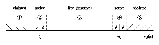
Illustration of the constraints lj≤rjx≤uj

Figure 1: Illustration of the constraints $l_{j} \leq r_{j} (x) \leq u_{j}$

If there are no nonlinear constraints in (1) and

F

is linear or quadratic, then it will generally be more efficient to use one of e04mf, e04nc or e04nf. If the problem is large and sparse and does have nonlinear constraints, then e04vh should be used, since e04wd treats all matrices as dense.

You must supply an initial estimate of the solution to (1), together with methods that define

F (x)

and

c (x)

with as many first partial derivatives as possible; unspecified derivatives are approximated by finite differences; see [Description of the Optional Parameters] for a discussion of the optional parameter Derivative Level.

The objective function is defined by objfun, and the nonlinear constraints are defined by confun. Note that if there are any nonlinear constraints then the first call to confun will precede the first call to objfun.

For maximum reliability, it is preferable for you to provide all partial derivatives (see Chapter 8 of Gill et al. (1981), for a detailed discussion). If all gradients cannot be provided, it is similarly advisable to provide as many as possible. While developing objfun and confun, the optional parameter Verify Level should be used to check the calculation of any known gradients.

The method used by e04wd is based on NPOPT, which is part of the SNOPT package described in Gill et al. (2005b), and the algorithm it uses is described in detail in [Algorithmic Details].

References

Eldersveld S K (1991) Large-scale sequential quadratic programming algorithms PhD Thesis Department of Operations Research, Stanford University, Stanford

Fourer R (1982) Solving staircase linear programs by the simplex method Math. Programming 23 274–313

Gill P E, Murray W and Saunders M A (2002) SNOPT: An SQP Algorithm for Large-scale Constrained Optimization 12 979–1006 SIAM J. Optim.

Gill P E, Murray W and Saunders M A (2005a) Users' guide for SQOPT 7: a Fortran package for large-scale linear and quadratic programming Report NA 05-1 Department of Mathematics, University of California, San Diego http://www.ccom.ucsd.edu/~peg/papers/sqdoc7.pdf

Gill P E, Murray W and Saunders M A (2005b) Users' guide for SNOPT 7.1: a Fortran package for large-scale linear nonlinear programming Report NA 05-2 Department of Mathematics, University of California, San Diego http://www.ccom.ucsd.edu/~peg/papers/sndoc7.pdf

Gill P E, Murray W, Saunders M A and Wright M H (1986) Users' guide for NPSOL (Version 4.0): a Fortran package for nonlinear programming Report SOL 86-2 Department of Operations Research, Stanford University

Gill P E, Murray W, Saunders M A and Wright M H (1992) Some theoretical properties of an augmented Lagrangian merit function Advances in Optimization and Parallel Computing (ed P M Pardalos) 101–128 North Holland

Gill P E, Murray W and Wright M H (1981) Practical Optimization Academic Press

Hock W and Schittkowski K (1981) Test Examples for Nonlinear Programming Codes. Lecture Notes in Economics and Mathematical Systems 187 Springer–Verlag

Error Indicators and Warnings

Note: e04wd may return useful information for one or more of the following detected errors or warnings.

Errors or warnings detected by the method:

Some error messages may refer to parameters that are dropped from this interface (LDA, LDCJ, LDH) In these cases, an error in another parameter has usually caused an incorrect value to be inferred.

$ifail = 1$: The initialization method (E04WCF not in this release) has not been called or at least one of leniw and lenrw is less than $600$ .

$ifail = 2$: An input parameter is invalid. The output message provides more details of the invalid argument.

$ifail = 3$: Requested accuracy could not be achieved.
A feasible solution has been found, but the requested accuracy in the dual infeasibilities could not be achieved. An abnormal termination has occurred, but e04wd is within $10^{- 2}$ of satisfying the Major Optimality Tolerance. Check that the Major Optimality Tolerance is not too small.

$ifail = 4$: The problem appears to be infeasible.
When the constraints are linear, this message is based on a relatively reliable indicator of infeasibility. Feasibility is measured with respect to the upper and lower bounds on the variables and slacks. Among all the points satisfying the general constraints $A x - s = 0$ (see (5) and (6) in [Major Iterations]), there is apparently no point that satisfies the bounds on $x$ and $s$ . Violations as small as the Minor Feasibility Tolerance are ignored, but at least one component of $x$ or $s$ violates a bound by more than the tolerance.
When nonlinear constraints are present, infeasibility is much harder to recognize correctly. Even if a feasible solution exists, the current linearization of the constraints may not contain a feasible point. In an attempt to deal with this situation, when solving each QP subproblem, e04wd is prepared to relax the bounds on the slacks associated with nonlinear rows.
If a QP subproblem proves to be infeasible or unbounded (or if the Lagrange multiplier estimates for the nonlinear constraints become large), e04wd enters so-called ‘nonlinear elastic’ mode. The subproblem includes the original QP objective and the sum of the infeasibilities – suitably weighted using the optional parameter Elastic Weight. In elastic mode, some of the bounds on the nonlinear rows are ‘elastic’ – i.e., they are allowed to violate their specific bounds. Variables subject to elastic bounds are known as elastic variables. An elastic variable is free to violate one or both of its original upper or lower bounds. If the original problem has a feasible solution and the elastic weight is sufficiently large, a feasible point eventually will be obtained for the perturbed constraints, and optimization can continue on the subproblem. If the nonlinear problem has no feasible solution, e04wd will tend to determine a ‘good’ infeasible point if the elastic weight is sufficiently large. (If the elastic weight were infinite, e04wd would locally minimize the nonlinear constraint violations subject to the linear constraints and bounds.)
Unfortunately, even though e04wd locally minimizes the nonlinear constraint violations, there may still exist other regions in which the nonlinear constraints are satisfied. Wherever possible, nonlinear constraints should be defined in such a way that feasible points are known to exist when the constraints are linearized.

$ifail = 5$: The problem appears to be unbounded (or badly scaled).
For linear problems, unboundedness is detected by the simplex method when a nonbasic variable can be increased or decreased by an arbitrary amount without causing a basic variable to violate a bound. Consider adding an upper or lower bound to the variable. Also, examine the constraints that have nonzeros in the associated column, to see if they have been formulated as intended.
Very rarely, the scaling of the problem could be so poor that numerical error will give an erroneous indication of unboundedness. Consider using the optional parameter Scale Option.
For nonlinear problems, e04wd monitors both the size of the current objective function and the size of the change in the variables at each step. If either of these is very large (as judged by the unbounded parameters (see [Major Iteration Log])), the problem is terminated and declared unbounded. To avoid large function values, it may be necessary to impose bounds on some of the variables in order to keep them away from singularities in the nonlinear functions.
The message may indicate an abnormal termination while enforcing the limit on the constraint violations. This exit implies that the objective is not bounded below in the feasible region defined by expanding the bounds by the value of the Violation Limit.

$ifail = 6$: Iteration limit reached.
Either the Iterations Limit or the Major Iterations Limit was exceeded before the required solution could be found. Check the iteration log to be sure that progress was being made. If so, and if you caused a basis file to be saved by using the optional parameter New Basis File, consider restarting the run using the optional parameter Old Basis File to see whether further progress can be made. If you have no basis file available, you might rerun the problem after increasing the optional parameters Minor Iterations Limit and/or Major Iterations Limit.
If none of the above limits have been reached, this error may mean that the problem appears to be more nonlinear than anticipated. The current set of basic and superbasic variables have been optimized as much as possible and a pricing operation (where a nonbasic variable is selected to become superbasic) is necessary to continue, but it can't continue as the number of superbasic variables has already reached the limit specified by the optional parameter Superbasics Limit. In general, raise the Superbasics Limit $s$ by a reasonable amount, bearing in mind the storage needed for the reduced Hessian. (The Reduced Hessian Dimension $h$ will also increase to $s$ unless specified otherwise, and the associated storage will be about $\frac{1}{2} s^{2}$ words.) In some cases you may have to set $h < s$ to conserve storage, but beware that the rate of convergence will probably fall off severely.

$ifail = 7$

Numerical difficulties have been encountered and no further progress can be made.

Several circumstances could lead to this exit.

1.	The user-supplied delegates objfun or confun could be returning accurate function values but inaccurate gradients (or vice versa). This is the most likely cause. Study the comments given for $ifail = 8$ , and do your best to ensure that the coding is correct.
2.	The function and gradient values could be consistent, but their precision could be too low. For example, accidental use of a real data type when double precision was intended would lead to a relative function precision of about $10^{- 6}$ instead of something like $10^{- 15}$ . The default Major Optimality Tolerance of $2 \times 10^{- 6}$ would need to be raised to about $10^{- 3}$ for optimality to be declared (at a rather suboptimal point). Of course, it is better to revise the function coding to obtain as much precision as economically possible.
3.	If function values are obtained from an expensive iterative process, they may be accurate to rather few significant figures, and gradients will probably not be available. One should specify Function Precision $t$ Major Optimality Tolerance $\sqrt{t}$ but even then, if $t$ is as large as $10^{- 5}$ or $10^{- 6}$ (only $5$ or $6$ significant figures), the same exit condition may occur. At present the only remedy is to increase the accuracy of the function calculation.
4.	An $L U$ factorization of the basis has just been obtained and used to recompute the basic variables $x_{B}$ , given the present values of the superbasic and nonbasic variables. A step of ‘iterative refinement’ has also been applied to increase the accuracy of $x_{B}$ . However, a row check has revealed that the resulting solution does not satisfy the current constraints $A x - s = 0$ sufficiently well. This probably means that the current basis is very ill-conditioned. If there are some linear constraints and variables, try $Scale Option = 1$ if scaling has not yet been used. For certain highly structured basis matrices (notably those with band structure), a systematic growth may occur in the factor $U$ . Consult the description of Umax and Growth in [Basis Factorization Statistics] and set the LU Factor Tolerance to $2.0$ (or possibly even smaller, but not less than $1.0$ ).
5.	The first factorization attempt will have found the basis to be structurally or numerically singular. (Some diagonals of the triangular matrix $U$ were respectively zero or smaller than a certain tolerance.) The associated variables are replaced by slacks and the modified basis is refactorized, but singularity persists. This must mean that the problem is badly scaled, or the LU Factor Tolerance is too much larger than $1.0$ . This is highly unlikely to occur.

$ifail = 8$: Derivative appears to be incorrect.
If the message refers to the derivatives of the objective function, then a check has been made on some individual elements of the objective gradient array at the first point that satisfies the linear constraints. At least one component $grad j - 1$ is being set to a value that disagrees markedly with its associated forward-difference estimate $\frac{\partial F}{\partial x_{j}}$ . (The relative difference between the computed and estimated values is $1.0$ or more.) This exit is a safeguard, since e04wd will usually fail to make progress when the computed gradients are seriously inaccurate. In the process it may expend considerable effort before terminating with $ifail = 7$ .
Check the function and gradient computation very carefully in objfun. A simple omission could explain everything. If $F$ or a component $\frac{\partial F}{\partial x_{j}}$ is very large, then give serious thought to scaling the function or the nonlinear variables.
If you feel certain that the computed $grad [j - 1]$ is correct (and that the forward-difference estimate is therefore wrong), you can specify $Verify Level = 0$ to prevent individual elements from being checked. However, the optimization procedure may have difficulty.
If the message refers to derivatives of the constraints, then at least one of the computed constraint derivatives is significantly different from an estimate obtained by forward-differencing the vector $c (x)$ . Follow the advice given above, trying to ensure that the arrays ccon and cjac are being set correctly in confun.

$ifail = 9$

Undefined user-supplied function.

You have indicated that the problem functions are undefined by assigning the value

mode = - 1

on exit from objfun or confun. e04wd attempts to evaluate the problem functions closer to a point at which the functions are already known to be defined. This exit occurs if e04wd is unable to find a point at which the functions are defined. This will occur in the case of:

–	undefined functions with no recovery possible;
–	undefined functions at the first point;
–	undefined functions at the first feasible point; or
–	undefined functions when checking derivatives.

$ifail = 10$: User requested termination.
You have indicated the wish to terminate solution of the current problem by setting mode to a value $< - 1$ on exit from objfun or confun.

$ifail = 11$: Internal memory allocation failed when attempting to obtain the required workspace. Please contact NAG.

$ifail = 12$: Internal memory allocation was insufficient. Please contact NAG.

$ifail = 13$: An error has occurred in the basis package, perhaps indicating incorrect setup of arrays. Set the optional parameter Print File and examine the output carefully for further information.

$ifail = 14$: An unexpected error has occurred. Set the optional parameter Print File and examine the output carefully for further information.

$ifail = -9000$: An error occured, see message report.
$ifail = -6000$: Invalid Parameters $〈value〉$
$ifail = -4000$: Invalid dimension for array $〈value〉$
$ifail = -8000$: Negative dimension for array $〈value〉$
$ifail = -6000$: Invalid Parameters $〈value〉$

Accuracy

ifail = 0

on exit, then the vector returned in the array x is an estimate of the solution to an accuracy of approximately Major Optimality Tolerance.

Parallelism and Performance

None.

Further Comments

This section describes the final output produced by e04wd. Intermediate and other output are given in [Description of Monitoring Information].

The Final Output

Print File > 0

, the final output, including a listing of the status of every variable and constraint will be sent to the channel numbers associated with Print File. The following describes the output for each variable. A full stop (.) is printed for any numerical value that is zero.

Variable

gives the name (Variable) and index

j

, for

j = 1, 2, \dots, n

, of the variable.

State

gives the state of the variable (FR if neither bound is in the working set, EQ if a fixed variable, LL if on its lower bound, UL if on its upper bound, TF if temporarily fixed at its current value). If Value lies outside the upper or lower bounds by more than the Feasibility Tolerance, State will be ++ or -- respectively. (The latter situation can occur only when there is no feasible point for the bounds and linear constraints.)

A key is sometimes printed before State.

A	Alternative optimum possible. The variable is active at one of its bounds, but its Lagrange multiplier is essentially zero. This means that if the variable were allowed to start moving away from its bound then there would be no change to the objective function. The values of the other free variables might change, giving a genuine alternative solution. However, if there are any degenerate variables (labelled D), the actual change might prove to be zero, since one of them could encounter a bound immediately. In either case the values of the Lagrange multipliers might also change.
D	Degenerate. The variable is free, but it is equal to (or very close to) one of its bounds.
I	Infeasible. The variable is currently violating one of its bounds by more than the Feasibility Tolerance.

Value

is the value of the variable at the final iteration.

Lower bound

is the lower bound specified for the variable. None indicates that

bl [j - 1] \leq - bigbnd

Upper bound

is the upper bound specified for the variable. None indicates that

bu [j - 1] \geq bigbnd

Lagr multiplier

is the Lagrange multiplier for the associated bound. This will be zero if State is FR unless

bl [j - 1] \leq - bigbnd

and

bu [j - 1] \geq bigbnd

, in which case the entry will be blank. If

x

is optimal, the multiplier should be non-negative if State is LL and non-positive if State is UL.

Slack

is the difference between the variable Value and the nearer of its (finite) bounds

bl [j - 1]

and

bu [j - 1]

. A blank entry indicates that the associated variable is not bounded (i.e.,

bl [j - 1] \leq - bigbnd

and

bu [j - 1] \geq bigbnd

The meaning of the output for linear and nonlinear constraints is the same as that given above for variables, with

bl [j - 1]

and

bu [j - 1]

replaced by

bl [n + j - 1]

and

bu [n + j - 1]

respectively, and with the following changes in the heading:

Linear constrnt	gives the name (lincon) and index $j$ , for $j = 1, 2, \dots, n_{L}$ , of the linear constraint.
Nonlin constrnt	gives the name (nlncon) and index ( $j - n_{L}$ ), for $j = n_{L} + 1, \dots, n_{L} + n_{N}$ , of the nonlinear constraint.

Note that movement off a constraint (as opposed to a variable moving away from its bound) can be interpreted as allowing the entry in the Slack column to become positive.

Numerical values are output with a fixed number of digits; they are not guaranteed to be accurate to this precision.

Example

This example is based on Problem 71 in Hock and Schittkowski (1981) and involves the minimization of the nonlinear function

F (x) = x_{1} x_{4} (x_{1} + x_{2} + x_{3}) + x_{3}

subject to the bounds

\begin{array}{l} 1 \leq x_{1} \leq 5 \\ 1 \leq x_{2} \leq 5 \\ 1 \leq x_{3} \leq 5 \\ 1 \leq x_{4} \leq 5, \end{array}

to the general linear constraint

x_{1} + x_{2} + x_{3} + x_{4} \leq 20,

and to the nonlinear constraints

\begin{matrix} x_{1}^{2} + x_{2}^{2} + x_{3}^{2} + x_{4}^{2} \leq 40, \\ x_{1} x_{2} x_{3} x_{4} \geq 25 . \end{matrix}

The initial point, which is infeasible, is

x_{0} = {(1, 5, 5, 1)}^{T},

with

F (x_{0}) = 16

The optimal solution (to five figures) is

x^{*} = {(1.0, 4.7430, 3.8211, 1.3794)}^{T},

and

F (x^{*}) = 17.014

. One bound constraint and both nonlinear constraints are active at the solution.

Example program (C#): e04wde.cs

Example program data: e04wde.d

Example program results: e04wde.r

Algorithmic Details

Here we summarise the main features of the SQP algorithm used in e04wd and introduce some terminology used in the description of the method and its arguments. The SQP algorithm is fully described in Gill et al. (2002).

Constraints and Slack Variables

The upper and lower bounds on the

n_{L} + n_{N}

components of

(\begin{matrix} A_{L} x \\ c (x) \end{matrix})

are said to define the general constraints of the problem. e04wd converts the general constraints to equalities by introducing a set of slack variables

s = {(s_{1}, s_{2}, \dots, s_{n_{L} + n_{N}})}^{T}

. For example, the linear constraint

5 \leq 2 x_{1} + 3 x_{2} \leq \infty

is replaced by

2 x_{1} + 3 x_{2} - s_{1} = 0

together with the bounded slack

5 \leq s_{1} \leq \infty

. The minimization problem (1) can therefore be written in the equivalent form

\underset{x, s}{minimize} F (x) subject to ​ (\begin{matrix} A_{L} x \\ c (x) \end{matrix}) - s = 0, l \leq (\begin{matrix} x \\ s \end{matrix}) \leq u .

(2)

The general constraints become the equalities

A_{L} x - s_{L} = 0

and

c (x) - s_{N} = 0

, where

s_{L}

and

s_{N}

are the linear and nonlinear slacks.

Major Iterations

The basic structure of the SQP algorithm involves major and minor iterations. The major iterations generate a sequence of iterates

\{x_{k}\}

that satisfy the linear constraints and converge to a point that satisfies the nonlinear constraints and the first-order conditions for optimality. At each iterate

x_{k}

a QP subproblem is used to generate a search direction towards the next iterate

x_{k + 1}

. The constraints of the subproblem are formed from the linear constraints

A_{L} x - s_{L} = 0

and the linearized constraint

c (x_{k}) + c^{'} (x_{k}) (x - x_{k}) - s_{N} = 0,

(3)

where

c^{'} (x_{k})

denotes the Jacobian matrix, whose elements are the first derivatives of

c (x)

evaluated at

x_{k}

. The QP constraints therefore comprise the

n_{L} + n_{N}

linear constraints

\begin{array}{l} A_{L} x - s_{L} & = & 0, \\ c^{'} (x_{k}) x - s_{N} & = & - c (x_{k}) + c^{'} (x_{k}) x_{k}, \end{array}

(4)

where

x

and

s

are bounded above and below by

u

and

l

as before. If the

(n_{L} + n_{N}) \times n

matrix

A

and

(n_{L} + n_{N})

-vector

b

are defined as

A = (\begin{matrix} A_{L} \\ c^{'} (x_{k}) \end{matrix}) and b = (\begin{matrix} 0 \\ - c (x_{k}) + c^{'} (x_{k}) x_{k} \end{matrix}),

(5)

then the QP subproblem can be written as

\underset{x, s}{minimize} q (x, x_{k}) = g_{k}^{T} (x - x_{k}) + \frac{1}{2} (x - x_{k}) H_{k} (x - x_{k}) subject to ​ A x - s = b, l \leq (\begin{matrix} x \\ s \end{matrix}) \leq u,

(6)

where

q (x, x_{k})

is a quadratic approximation to a modified Lagrangian function (see Gill et al. (2002)). The matrix

H_{k}

is a quasi-Newton approximation to the Hessian of the Lagrangian. A BGFS update is applied after each major iteration. If some of the variables enter the Lagrangian linearly the Hessian will have some zero rows and columns. If the nonlinear variables appear first, then only the leading

n_{N}

rows and columns of the Hessian need to be approximated.

Minor Iterations

Solving the QP subproblem is itself an iterative procedure. Here, the iterations of the QP solver e04nq form the minor iterations of the SQP method. e04nq uses a reduced-Hessian active-set method implemented as a reduced-gradient method. At each minor iteration, the constraints

A x - s = b

are partitioned into the form

B x_{B} + S x_{S} + N x_{N} = b,

(7)

where the basis matrix

B

is square and nonsingular, and the matrices

S

and

N

are the remaining columns of

(\begin{matrix} A & - I \end{matrix})

. The vectors

x_{B}

x_{S}

and

x_{N}

are the associated basic, superbasic and nonbasic variables respectively; they are a permutation of the elements of

x

and

s

. At a QP subproblem, the basic and superbasic variables will lie somewhere between their bounds, while the nonbasic variables will normally be equal to one of their bounds. At each iteration,

x_{S}

is regarded as a set of independent variables that are free to move in any desired direction, namely one that will improve the value of the QP objective (or the sum of infeasibilities). The basic variables are then adjusted in order to ensure that

(x, s)

continues to satisfy

A x - s = b

. The number of superbasic variables (

n_{S}

, say) therefore indicates the number of degrees of freedom remaining after the constraints have been satisfied. In broad terms,

n_{S}

is a measure of how nonlinear the problem is. In particular,

n_{S}

will always be zero for LP problems.

If it appears that no improvement can be made with the current definition of

B

S

and

N

, a nonbasic variable is selected to be added to

S

, and the process is repeated with the value of

n_{S}

increased by one. At all stages, if a basic or superbasic variable encounters one of its bounds, the variable is made nonbasic and the value of

n_{S}

is decreased by one.

Associated with each of the

n_{L} + n_{N}

equality constraints

A x - s = b

are the dual variables

π

. Similarly, each variable in

(x, s)

has an associated reduced gradient

d_{j}

. The reduced gradients for the variables

x

are the quantities

g - A^{T} π

, where

g

is the gradient of the QP objective, and the reduced gradients for the slacks are the dual variables

π

. The QP subproblem is optimal if

d_{j} \geq 0

for all nonbasic variables at their lower bounds,

d_{j} \leq 0

for all nonbasic variables at their upper bounds, and

d_{j} = 0

for other variables, including superbasics. In practice, an approximate QP solution

({\hat{x}}_{k}, {\hat{s}}_{k}, {\hat{π}}_{k})

is found by relaxing these conditions.

The Merit Function

After a QP subproblem has been solved, new estimates of the solution are computed using a linesearch on the augmented Lagrangian merit function

M (x, s, π) = F (x) - π^{T} (c (x) - s_{N}) + \frac{1}{2} {(c (x) - s_{N})}^{T} D (c (x) - s_{N}),

(8)

where

D

is a diagonal matrix of penalty parameters

(D_{i i} \geq 0)

, and

π

now refers to dual variables for the nonlinear constraints in (1). If

(x_{k}, s_{k}, π_{k})

denotes the current solution estimate and

({\hat{x}}_{k}, {\hat{s}}_{k}, {\hat{π}}_{k})

denotes the QP solution, the linesearch determines a step

α_{k}

(0 < α_{k} \leq 1)

such that the new point

(\begin{matrix} x_{k + 1} \\ s_{k + 1} \\ π_{k + 1} \end{matrix}) = (\begin{matrix} x_{k} \\ s_{k} \\ π_{k} \end{matrix}) + α_{k} (\begin{matrix} {\hat{x}}_{k} - x_{k} \\ {\hat{s}}_{k} - s_{k} \\ {\hat{π}}_{k} - π_{k} \end{matrix})

(9)

gives a sufficient decrease in the merit function

M

. When necessary, the penalties in

D

are increased by the minimum-norm perturbation that ensures descent for

M

(see Gill et al. (1992)). The value of

s_{N}

is adjusted to minimize the merit function as a function of

s

before the solution of the QP subproblem (see Gill et al. (1986) and Eldersveld (1991)).

Treatment of Constraint Infeasibilities

e04wd makes explicit allowance for infeasible constraints. First, infeasible linear constraints are detected by solving the linear program

\underset{x, v, w}{minimize} e^{T} (v + w) subject to ​ l \leq (\begin{matrix} x \\ A_{L} x - v + w \end{matrix}) \leq u, v \geq 0, w \geq 0,

(10)

where

e

is a vector of ones, and the nonlinear constraint bounds are temporarily excluded from

l

and

u

. This is equivalent to minimizing the sum of the general linear constraint violations subject to the bounds on

x

. (The sum is the

ℓ_{1}

-norm of the linear constraint violations. In the linear programming literature, the approach is called elastic programming.)

The linear constraints are infeasible if the optimal solution of (10) has

v \neq 0

w \neq 0

. e04wd then terminates without computing the nonlinear functions.

Otherwise, all subsequent iterates satisfy the linear constraints. (Such a strategy allows linear constraints to be used to define a region in which the functions can be safely evaluated.) e04wd proceeds to solve nonlinear problems as given, using search directions obtained from the sequence of QP subproblems (see (6)).

If a QP subproblem proves to be infeasible or unbounded (or if the dual variables

π

for the nonlinear constraints become large), e04wd enters ‘elastic’ mode and thereafter solves the problem

\underset{x, v, w}{minimize} F (x) + γ e^{T} (v + w) subject to ​ l \leq (\begin{matrix} x \\ A_{L} x \\ c (x) - v + w \end{matrix}) \leq u, v \geq 0, w \geq 0,

(11)

where

γ

is a non-negative parameter (the elastic weight), and

F (x) + γ e^{T} (v + w)

is called a composite objective (the

ℓ_{1}

penalty function for the nonlinear constraints).

The value of

γ

may increase automatically by multiples of

10

if the optimal

v

and

w

continue to be nonzero. If

γ

is sufficiently large, this is equivalent to minimizing the sum of the nonlinear constraint violations subject to the linear constraints and bounds.

The initial value of

γ

is controlled by the optional parameter Elastic Weight.

Description of Monitoring Information

e04wd produces monitoring information, statistical information and information about the solution. [The Final Output] contains the final output information sent to unit Print File. This section contains other output information.

Major Iteration Log

This section describes the output to unit Print File if

Major Print Level > 0

. One line of information is output every

k

th major iteration, where

k

is Print Frequency.

Label	Description
Itns	is the cumulative number of minor iterations.
Major	is the current major iteration number.
Minors	is the number of iterations required by both the feasibility and optimality phases of the QP subproblem. Generally, Minors will be $1$ in the later iterations, since theoretical analysis predicts that the correct active set will be identified near the solution (see [Algorithmic Details]).
Step	is the step length $α$ taken along the current search direction $p$ . The variables $x$ have just been changed to $x + α p$ . On reasonably well-behaved problems, the unit step will be taken as the solution is approached.
nCon or nObj	nCon is the number of times confun has been called to evaluate the nonlinear problem functions. Evaluations needed for the estimation of the derivatives by finite differences are not included. nCon is printed as a guide to the amount of work required for the linesearch. If $n_{N}$ , the number of nonlinear constraints, is zero, nCon does not appear, but is replaced by nObj. This quantity is the number of calls made to objfun.
Feasible	is the value of $v_{\max}$ (see (12)), the maximum component of the scaled nonlinear constraint residual (see the description of the optional parameter Major Feasibility Tolerance). The solution is regarded as acceptably feasible if Feasible is less than the Major Feasibility Tolerance. In this case, the entry is contained in parentheses. If the constraints are linear, all iterates are feasible and this entry is not printed.
Optimal	is the value of $c_{\max}$ (see (13)), the maximum complementary gap (see the description of the optional parameter Major Optimality Tolerance). It is an estimate of the degree of nonoptimality of the reduced costs. Both Feasible and Optimal are small in the neighbourhood of a solution.
MeritFunction or Objective	is the value of the augmented Lagrangian merit function (see (8)). This function will decrease at each iteration unless it was necessary to increase the penalty parameters (see [The Merit Function]). As the solution is approached, MeritFunction will converge to the value of the objective at the solution. In elastic mode, the merit function is a composite function involving the constraint violations weighted by the elastic weight. If the constraints are linear, this item is labelled Objective, the value of the objective function. It will decrease monotonically to its optimal value.
L+U	is the number of nonzeros representing the basis factors $L$ and $U$ on completion of the QP subproblem. If nonlinear constraints are present, the basis factorization $B = L U$ is computed at the start of the first minor iteration. At this stage, $L+U = lenL + lenU$ , where lenL (see [Basis Factorization Statistics]) is the number of subdiagonal elements in the columns of a lower triangular matrix and lenU (see [Basis Factorization Statistics]) is the number of diagonal and superdiagonal elements in the rows of an upper-triangular matrix. As columns of $B$ are replaced during the minor iterations, L+U may fluctuate up or down but, in general, will tend to increase. As the solution is approached and the minor iterations decrease towards zero, L+U will reflect the number of nonzeros in the $L U$ factors at the start of the QP subproblem. If the constraints are linear, refactorization is subject only to the Factorization Frequency, and L+U will tend to increase between factorizations.
BSwap	is the number of columns of the basis matrix $B$ that were swapped with columns of $S$ to improve the condition of $B$ . The swaps are determined by an $L U$ factorization of the rectangular matrix $B_{S} = {(\begin{matrix} B & S \end{matrix})}^{T}$ with stability being favoured more than sparsity.
nS	is the current number of superbasic variables.
condHz	is an estimate of the condition number of $R^{T} R$ , itself an estimate of $Z^{T} H Z$ , the reduced Hessian of the Lagrangian. The condition number is the square of the ratio of the largest and smallest diagonals of the upper triangular matrix $R$ , this being a lower bound on the condition number of $R^{T} R$ . condHz gives a rough indication of whether or not the optimization procedure is having difficulty. If $ε$ is the relative machine precision being used, the SQP algorithm will make slow progress if condHz becomes as large as $ε^{- 1 / 2} \approx 10^{8}$ , and will probably fail to find a better solution if condHz reaches $ε^{- 3 / 4} \approx 10^{12}$ . To guard against high values of condHz, attention should be given to the scaling of the variables and the constraints. In some cases it may be necessary to add upper or lower bounds to certain variables to keep them a reasonable distance from singularities in the nonlinear functions or their derivatives.
Penalty	is the Euclidean norm of the vector of penalty parameters used in the augmented Lagrangian merit function (not printed if there are no nonlinear constraints).

The summary line may include additional code characters that indicate what happened during the course of the major iteration. These will follow the separator ‘_’ in the output.

Label	Description
c	central differences have been used to compute the unknown components of the objective and constraint gradients. A switch to central differences is made if either the linesearch gives a small step, or $x$ is close to being optimal. In some cases, it may be necessary to re-solve the QP subproblem with the central difference gradient and Jacobian.
d	during the linesearch it was necessary to decrease the step in order to obtain a maximum constraint violation conforming to the value of Violation Limit.
D	you set $mode = - 1$ on exit from objfun, indicating that the linesearch needed to be done with a smaller value of the step length $α$ .
l	the norm wise change in the variables was limited by the value of the Major Step Limit. If this output occurs repeatedly during later iterations, it may be worthwhile increasing the value of Major Step Limit.
i	if e04wd is not in elastic mode, an i signifies that the QP subproblem is infeasible. This event triggers the start of nonlinear elastic mode, which remains in effect for all subsequent iterations. Once in elastic mode, the QP subproblems are associated with the elastic problem (11) (see [Treatment of Constraint Infeasibilities]). If e04wd is already in elastic mode, an i indicates that the minimizer of the elastic subproblem does not satisfy the linearized constraints. (In this case, a feasible point for the usual QP subproblem may or may not exist.)
M	an extra evaluation of the problem functions was needed to define an acceptable positive definite quasi-Newton update to the Lagrangian Hessian. This modification is only done when there are nonlinear constraints.
m	this is the same as M except that it was also necessary to modify the update to include an augmented Lagrangian term.
n	no positive definite BFGS update could be found. The approximate Hessian is unchanged from the previous iteration.
R	the approximate Hessian has been reset by discarding all but the diagonal elements. This reset will be forced periodically by the Hessian Frequency and Hessian Updates keywords. However, it may also be necessary to reset an ill-conditioned Hessian from time to time.
r	the approximate Hessian was reset after ten consecutive major iterations in which no BFGS update could be made. The diagonals of the approximate Hessian are retained if at least one update has been done since the last reset. Otherwise, the approximate Hessian is reset to the identity matrix.
s	a self-scaled BFGS update was performed. This update is used when the Hessian approximation is diagonal, and hence always follows a Hessian reset.
t	the minor iterations were terminated because of the Minor Iterations Limit.
T	the minor iterations were terminated because of the New Superbasics Limit.
u	the QP subproblem was unbounded.
w	a weak solution of the QP subproblem was found.
z	the Superbasics Limit was reached.

Minor Iteration Log

Minor Print Level > 0

, one line of information is output to the Print file every

k

th minor iteration, where

k

is the specified Print Frequency. A heading is printed before the first such line following a basis factorization. The heading contains the items described below. In this description, a pricing operation is the process by which a nonbasic variable is selected to become superbasic (in addition to those already in the superbasic set). The selected variable is denoted by jq. Variable jq often becomes basic immediately. Otherwise it remains superbasic, unless it reaches its opposite bound and returns to the nonbasic set.

If Partial Price is in effect, variable jq is selected from

A_{pp}

I_{pp}

, the

pp

th segments of the constraint matrix

(\begin{matrix} A & - I \end{matrix})

Label	Description
Itn	the current iteration number.
LPmult or QPmult	is the reduced cost (or reduced gradient) of the variable jq selected by the pricing procedure at the start of the present iteration. Algebraically, the reduced gradient is $d_{j} = g_{j} - π^{T} a_{j}$ for $j = jq$ , where $g_{j}$ is the gradient of the current objective function, $π$ is the vector of dual variables for the QP subproblem, and $a_{j}$ is the $j$ th column of $(\begin{matrix} A & - I \end{matrix})$ . Note that the reduced cost is the $1$ -norm of the reduced-gradient vector at the start of the iteration, just after the pricing procedure.
LPstep or QPstep	is the step length $α$ taken along the current search direction $p$ . The variables $x$ have just been changed to $x + α p$ . Write Step to stand for LPStep or QPStep, depending on the problem. If a variable is made superbasic during the current iteration ( $+SBS > 0$ ), Step will be the step to the nearest bound. During the solution of (11), the step can be greater than one only if the reduced Hessian is not positive definite.
nInf	is the number of infeasibilities after the present iteration. This number will not increase unless the iterations are in elastic mode.
SumInf	is the sum of infeasibilities after the present iteration, if $nInf > 0$ . The value usually decreases at each nonzero Step, but if it decreases by $2$ or more, SumInf may occasionally increase.
rgNorm	is the norm of the reduced-gradient vector at the start of the iteration. (It is the norm of the vector with elements $d_{j}$ for variables $j$ in the superbasic set.) During the solution of subproblem (11) this norm will be approximately zero after a unit step. (The heading is not printed if the problem is linear.)
LPobjective, QPobjective or Elastic QPobj	the QP objective function after the present iteration. In elastic mode, the heading is changed to Elastic QPobj. In either case, the value printed decreases monotonically.
+SBS	is the variable jq selected by the pricing operation to be added to the superbasic set.
-SBS	is the superbasic variable chosen to become nonbasic.
-BS	is the basis variable removed (if any) to become nonbasic.
Pivot	if column $a_{q}$ replaces the $r$ th column of the basis $B$ , Pivot is the $r$ th element of a vector $y$ satisfying $B y = a_{q}$ . Wherever possible, Step is chosen to avoid extremely small values of Pivot (since they cause the basis to be nearly singular). In rare cases, it may be necessary to increase the Pivot Tolerance to exclude very small elements of $y$ from consideration during the computation of Step.
L+U	is the number of nonzeros representing the basis factors $L$ and $U$ . Immediately after a basis factorization $B = L U$ , L+U is lenL+lenU, the number of subdiagonal elements in the columns of a lower triangular matrix and the number of diagonal and superdiagonal elements in the rows of an upper-triangular matrix. Further nonzeros are added to L when various columns of $B$ are later replaced. As columns of $B$ are replaced, the matrix $U$ is maintained explicitly (in sparse form). The value of L will steadily increase, whereas the value of U may fluctuate up or down. Thus the value of L+U may fluctuate up or down (in general, it will tend to increase).
ncp	is the number of compressions required to recover storage in the data structure for $U$ . This includes the number of compressions needed during the previous basis factorization.
nS	is the current number of superbasic variables. (The heading is not printed if the problem is linear.)
condHz	see [Major Iteration Log]. (The heading is not printed if the problem is linear.)

Crash Statistics

Major Print Level \geq 10

and System Information Yes has been specified, the following items are output to the Print file when Cold Start and no Backup Basis file is loaded. They refer to the number of columns that the Crash procedure selects during selected passes through

A

while searching for a triangular basis matrix.

Label	Description
Slacks	is the number of slacks selected initially.
Free cols	is the number of free columns in the basis.
Preferred	is the number of ‘preferred’ columns in the basis (i.e., $istate [j - 1] = 3$ for some $j \leq n$ ).
Unit	is the number of unit columns in the basis.
Double	is the number of columns in the basis containing $2$ nonzeros.
Triangle	is the number of triangular columns in the basis.
Pad	is the number of slacks used to pad the basis (to make it a nonsingular triangle).

Basis Factorization Statistics

Major Print Level \geq 10

, the first seven items in the list below are output to the Print file whenever the basis

B

or the rectangular matrix

B_{S} = {(\begin{matrix} B & S \end{matrix})}^{T}

is factorized before solution of the next QP subproblem. See [Description of the Optional Parameters] for a full description of an optional parameter.

Gaussian elimination is used to compute a sparse

L U

factorization of

B

B_{S}

, where

P L P^{T}

and

P U Q

are lower and upper triangular matrices for some permutation matrices

P

and

Q

. Stability is ensured as described under the optional parameter LU Factor Tolerance.

Minor Print Level \geq 10

, the same items are printed during the QP solution whenever the current

B

is factorized. In addition, if System Information Yes has been specified, the entries from Elems onwards are also printed.

Label

Description

Factor

the number of factorizations since the start of the run.

Demand

a code giving the reason for the present factorization, as follows:

Code	Meaning
0	First $L U$ factorization.
1	The number of updates reached the Factorization Frequency.
2	The nonzeros in the updated factors have increased significantly.
7	Not enough storage to update factors.
10	Row residuals too large (see the description of the optional parameter Check Frequency).
11	Ill-conditioning has caused inconsistent results.

Itn

is the current minor iteration number.

Nonlin

is the number of nonlinear variables in the current basis

B

Linear

is the number of linear variables in

B

Slacks

is the number of slack variables in

B

B BR BS or BT factorize

is the type of

L U

factorization.

B	periodic factorization of the basis $B$ .
BR	more careful rank-revealing factorization of $B$ using threshold rook pivoting. This occurs mainly at the start, if the first basis factors seem singular or ill-conditioned. Followed by a normal B factorize.
BS	$B_{S}$ is factorized to choose a well-conditioned $B$ from the current $(B S)$ . Followed by a normal B factorize.
BT	same as BS except the current $B$ is tried first and accepted if it appears to be not much more ill-conditioned than after the previous BS factorize.

is the number of rows in

B

B_{S}

is the number of columns in

B

B_{S}

. Preceded by ‘=’ or ‘>’ respectively.

Elems

is the number of nonzero elements in

B

B_{S}

Amax

is the largest nonzero in

B

B_{S}

Density

is the percentage nonzero density of

B

B_{S}

Merit/MerRP/MerCP

is the average Markowitz merit count for the elements chosen to be the diagonals of

P U Q

. Each merit count is defined to be

(c - 1) (r - 1)

where

c

and

r

are the number of nonzeros in the column and row containing the element at the time it is selected to be the next diagonal. Merit is the average of n such quantities. It gives an indication of how much work was required to preserve sparsity during the factorization. If LU Complete Pivoting or LU Rook Pivoting has been selected, this heading is changed to MerCP, respectively MerRP.

lenL

is the number of nonzeros in

L

L+U

is the number of nonzeros representing the basis factors

L

and

U

. Immediately after a basis factorization

B = L U

, L+U is lenL+lenU, the number of subdiagonal elements in the columns of a lower triangular matrix and the number of diagonal and superdiagonal elements in the rows of an upper-triangular matrix. Further nonzeros are added to L when various columns of

B

are later replaced. As columns of

B

are replaced, the matrix

U

is maintained explicitly (in sparse form). The value of L will steadily increase, whereas the value of U may fluctuate up or down. Thus the value of L+U may fluctuate up or down (in general, it will tend to increase).

Cmpressns

is the number of times the data structure holding the partially factored matrix needed to be compressed to recover unused storage. Ideally this number should be zero. If it is more than

3

4

, the amount of workspace available to e04wd should be increased for efficiency.

Incres

is the percentage increase in the number of nonzeros in

L

and

U

relative to the number of nonzeros in

B

B_{S}

Utri

is the number of triangular rows of

B

B_{S}

at the top of

U

lenU

the number of nonzeros in

U

, including its diagonals.

Ltol

is the largest subdiagonal element allowed in

L

. This is the specified LU Factor Tolerance or a smaller value that is currently being used for greater stability.

Umax

the maximum nonzero element in

U

Ugrwth

is the ratio

Umax / Amax

, which ideally should not be substantially larger than

10.0

100.0

. If it is orders of magnitude larger, it may be advisable to reduce the LU Factor Tolerance to

5.0

4.0

3.0

2.0

, say (but bigger than

1.0

As long as Lmax is not large (say

5.0

or less),

\max (Amax, Umax) / DUmin

gives an estimate of the condition number

B

. If this is extremely large, the basis is nearly singular. Slacks are used to replace suspect columns of

B

and the modified basis is refactored.

Ltri

is the number of triangular columns of

B

B_{S}

at the left of

L

dense1

is the number of columns remaining when the density of the basis matrix being factorized reached

0.3

Lmax

is the actual maximum subdiagonal element in

L

(bounded by Ltol).

Akmax

is the largest nonzero generated at any stage of the

L U

factorization. (Values much larger than Amax indicate instability.) Akmax is not printed if LU Partial Pivoting is selected.

Agrwth

is the ratio

Akmax / Amax

. Values much larger than

100

(say) indicate instability. Growth is not printed if LU Partial Pivoting is selected.

bump

is the size of the block to be factorized nontrivially after the triangular rows and columns of

B

B_{S}

have been removed.

dense2

is the number of columns remaining when the density of the basis matrix being factorized reached

0.6

. (The Markowitz pivot strategy searches fewer columns at that stage.)

DUmax

is the largest diagonal of

P U Q

DUmin

is the smallest diagonal of

P U Q

condU

the ratio

DUmax / DUmin

, which estimates the condition number of

U

(and of

B

if Ltol is less than

5.0

, say).

The Solution File

At the end of a run, the final solution may be output as a Solution file, according to Solution File. Some header information appears first to identify the problem and the final state of the optimization procedure. A ROWS section and a COLUMNS section then follow, giving one line of information for each row and column. The format used is similar to certain commercial systems, though there is no industry standard.

In general, numerical values are output with format f16.5. The maximum record length is

111

characters, including the first (carriage-control) character.

To reduce clutter, a full stop (.) is printed for any numerical value that is exactly zero. The values

\pm 1

are also printed specially as

1.0

and

- 1.0

. Infinite bounds (

\pm 10^{20}

or larger) are printed as None.

A Solution file is intended to be read from disk by a self-contained program that extracts and saves certain values as required for possible further computation. Typically, the first

14

records would be ignored. Each subsequent record may be read . The end of the ROWS section is marked by a record that starts with a

1

and is otherwise blank. If this and the next

4

records are skipped, the COLUMNS section can then be read under the same format. (There should be no need for backspace statements.)

The ROWS section

General linear constraints take the form

l \leq A x \leq u

. The

i

th constraint is therefore of the form

α \leq ν_{i} x \leq β,

where

ν_{i}

is the

i

th row of

A

Internally, the constraints take the form

A x - s = 0

, where

s

is the set of slack variables (which happen to satisfy the bounds

l \leq s \leq u

). For the

i

th constraint it is the slack variable

s_{i}

that is directly available, and it is sometimes convenient to refer to its state. Nonlinear constraints

α \leq c_{i} (x) + v_{i} x \leq β

are treated similarly, except that the row activity and degree of infeasibility are computed directly from

c_{i} (x) + v_{i} x

rather than

s_{i}

. A fullstop (.) is printed for any numerical value that is exactly zero.

Label

Description

Number

is the value of

n + i

. (This is used internally to refer to

s_{i}

in the intermediate output.)

Row

gives the name of the

i

th row.

State

the state of the

i

th row relative to the bounds

α

and

β

. The various states possible are as follows:

LL	the row is at its lower limit, $α$ .
UL	the row is at its upper limit, $β$ .
EQ	the limits are the same ( $α = β$ ).
FR	$s_{i}$ is nonbasic and currently zero, even though it is free to take any value between its bounds $α$ and $β$ .
BS	$s_{i}$ is basic.
SBS	$s_{i}$ is superbasic.

A key is sometimes printed before State. Note that unless the optional parameter

Scale Option = 0

is specified, the tests for assigning a key are applied to the variables of the scaled problem.

A	Alternative optimum possible. The variable is nonbasic, but its reduced gradient is essentially zero. This means that if the variable were allowed to start moving away from its bound, there would be no change in the value of the objective function. The values of the other free variables might change, giving a genuine alternative solution. However, if there are any degenerate variables (labelled D), the actual change might prove to be zero, since one of them could encounter a bound immediately. In either case, the values of the Lagrange multipliers might also change.
D	Degenerate. The variable is basic or superbasic, but it is equal (or very close) to one of its bounds.
I	Infeasible. The variable is basic or superbasic and is currently violating one of its bounds by more than the value of the Feasibility Tolerance.
N	Not precisely optimal. The variable is nonbasic or superbasic. If the value of the reduced gradient for the variable exceeds the value of the optional parameter Major Optimality Tolerance, the solution would not be declared optimal because the reduced gradient for the variable would not be considered negligible.

Activity

is the value of

v_{i} x

(or

c_{i} (x) + v_{i} x

for nonlinear rows) at the final iterate.

Slack Activity

is the value by which the row differs from its nearest bound. (For the free row (if any), it is set to Activity.)

Lower Limit

α

, the lower bound on the row.

Upper Limit

β

, the upper bound on the row.

Dual Activity

is the value of the dual variable

π_{i}

(the Lagrange multiplier for the

i

th constraint). The full vector

π

always satisfies

B^{T} π = g_{B}

, where

B

is the current basis matrix and

g_{B}

contains the associated gradients for the current objective function. For FP problems,

π_{i}

is set to zero.

gives the index

i

of the

i

th row.

The COLUMNS section

Let the

j

th component of

x

be the variable

x_{j}

and assume that it satisfies the bounds

α \leq x_{j} \leq β

. A fullstop (.) is printed for any numerical value that is exactly zero.

Label

Description

Number

is the column number

j

. (This is used internally to refer to

x_{j}

in the intermediate output.)

Column

gives the name of

x_{j}

State

the state of

x_{j}

relative to the bounds

α

and

β

. The various states possible are as follows:

LL	$x_{j}$ is nonbasic at its lower limit, $α$ .
UL	$x_{j}$ is nonbasic at its upper limit, $β$ .
EQ	$x_{j}$ is nonbasic and fixed at the value $α = β$ .
FR	$x_{j}$ is nonbasic at some value strictly between its bounds: $α < x_{j} < β$ .
BS	$x_{j}$ is basic. Usually $α < x_{j} < β$ .
SBS	$x_{j}$ is superbasic. Usually $α < x_{j} < β$ .

A key is sometimes printed before State. Note that unless the optional parameter

Scale Option = 0

is specified, the tests for assigning a key are applied to the variables of the scaled problem.

A	Alternative optimum possible. The variable is nonbasic, but its reduced gradient is essentially zero. This means that if the variable were allowed to start moving away from its bound, there would be no change in the value of the objective function. The values of the other free variables might change, giving a genuine alternative solution. However, if there are any degenerate variables (labelled D), the actual change might prove to be zero, since one of them could encounter a bound immediately. In either case, the values of the Lagrange multipliers might also change.
D	Degenerate. The variable is basic or superbasic, but it is equal (or very close) to one of its bounds.
I	Infeasible. The variable is basic or superbasic and is currently violating one of its bounds by more than the value of the Feasibility Tolerance.
N	Not precisely optimal. The variable is nonbasic or superbasic. If the value of the reduced gradient for the variable exceeds the value of the optional parameter Major Optimality Tolerance, the solution would not be declared optimal because the reduced gradient for the variable would not be considered negligible.

Activity

is the value of

x_{j}

at the final iterate.

Obj Gradient

is the value of

g_{j}

at the final iterate. For FP problems,

g_{j}

is set to zero.

Lower Limit

is the lower bound specified for the variable. None indicates that

bl [j - 1] \leq - bigbnd

Upper Limit

is the upper bound specified for the variable. None indicates that

bu [j - 1] \geq bigbnd

Reduced Gradnt

is the value of the reduced gradient

d_{j} = g_{j} - π^{T} a_{j}

where

a_{j}

is the

j

th column of the constraint matrix. For FP problems,

d_{j}

is set to zero.

m + j

is the value of

m + j

Note that movement off a constraint (as opposed to a variable moving away from its bound) can be interpreted as allowing the entry in the Slack Activity column to become positive.

Numerical values are output with a fixed number of digits; they are not guaranteed to be accurate to this precision.

The Summary File

Summary File > 0

, the following information is output to the unit number associated with Summary File. (It is a brief summary of the output directed to unit Print File):

–	the optional parameters supplied via the option setting methods, if any;
–	the Basis file loaded, if any;
–	a brief major iteration log (see [Major Iteration Log]);
–	a brief minor iteration log (see [Minor Iteration Log]);
–	the exit condition, ifail;
–	a summary of the final iterate.

Syntax

Parameters

Description

References

Error Indicators and Warnings

Accuracy

Parallelism and Performance

Further Comments

The Final Output

Example

Algorithmic Details

Constraints and Slack Variables

Major Iterations

Minor Iterations

The Merit Function

Treatment of Constraint Infeasibilities

Description of Monitoring Information

Major Iteration Log

Minor Iteration Log

Crash Statistics

Basis Factorization Statistics

The Solution File

The ROWS section

The COLUMNS section

The Summary File

See Also