NAG Library Chapter Introduction
G03 – Multivariate Methods
1 Scope of the Chapter
This chapter is concerned with methods for studying multivariate data. A multivariate dataset consists of several variables recorded on a number of objects or individuals. Multivariate methods can be classified as those that seek to examine the relationships between the variables (e.g., principal components), known as variable-directed methods, and those that seek to examine the relationships between the objects (e.g., cluster analysis), known as individual-directed methods.
Multiple regression is not included in this chapter as it involves the relationship of a single variable, known as the response variable, to the other variables in the dataset, the explanatory variables. Routines for multiple regression are provided in
Chapter G02.
2 Background to the Problems
2.1 Variable-directed Methods
Let the by data matrix consist of variables, , observed on objects or individuals. Variable-directed methods seek to examine the linear relationships between the variables with the aim of reducing the dimensionality of the problem. There are different methods depending on the structure of the problem. Principal component analysis and factor analysis examine the relationships between all the variables. If the individuals are classified into groups, then canonical variate analysis examines the between group structure. If the variables can be considered as coming from two sets, then canonical correlation analysis examines the relationships between the two sets of variables. All four methods are based on an eigenvalue decomposition or a singular value decomposition (SVD) of an appropriate matrix.
The above methods may reduce the dimensionality of the data from the original variables to a smaller number, , of derived variables that adequately represent the data. In general, these derived variables will be unique only up to an orthogonal rotation. Therefore, it may be useful to see if there exists suitable rotations of these variables that lead to a simple interpretation of the new variables in terms of the original variables.
2.1.1 Principal component analysis
Principal component analysis finds new variables which are linear combinations of the observed variables so that they have maximum variation and are orthogonal (uncorrelated).
Let
be the
by
variance-covariance matrix of the
by
data matrix. A vector
of length
is found such that
The variable
is known as the first principal component and gives the linear combination of the variables that gives the maximum variation. A second principal component,
, is found such that
This gives the linear combination of variables, orthogonal to the first principal component, that gives the maximum variation. Further principal components are derived in a similar way.
The vectors , for , are the eigenvectors of the matrix and associated with each eigenvector is the eigenvalue, . The value of gives the proportion of variation explained by the th principal component. Alternatively, the can be considered as the right singular vectors in a SVD of a scaled mean-centred data matrix. The singular values of the SVD are the -values.
Often fewer than dimensions (principal components) are needed to represent most of the variation in the data. A test on the smaller eigenvalues can be used to investigate the number of dimensions needed.
The values of the principal component variables for the individuals are known as the principal component scores. These can be standardized so that the variance of these scores for each principal component is or equal to the corresponding eigenvalue. The principal component scores correspond to the left-hand singular vectors in the SVD.
2.1.2 Factor analysis
Let the
variables have variance-covariance matrix
. The aim of factor analysis is to account for the covariances in these
variables in terms of a smaller number,
, of hypothetical variables or factors,
. These are assumed to be independent and to have unit variance. The relationship between the observed variables and the factors is given by the model
where
, for
and
, are the factor loadings and
, for
, are independent random variables with variances
. These represent the unique component of the variation of each observed variable. The proportion of variation for each variable accounted for by the factors is known as the communality.
The model for the variance-covariance matrix,
, can then be written as
where
is the matrix of the factor loadings,
, and
is a diagonal matrix of the unique variances
.
If it is assumed that both the
factors and the
follow independent Normal distributions then the parameters of the model,
and
, can be estimated by maximum likelihood, as described by
Lawley and Maxwell (1971). The computation of the maximum likelihood estimates is an iterative procedure which involves computing the eigenvalues and eigenvectors of the matrix
where
is the sample variance-covariance matrix. Alternatively, the SVD of the matrix
can be used, where
. When convergence has been achieved, the estimates
, of
, are obtained by scaling the eigenvectors of
. The use of maximum likelihood estimation means that likelihood ratio tests can be constructed to test for the number of factors required.
Having found the estimates of the parameters of the model, the estimates of the values of the factors for the individuals, the
factor
scores, can be computed. These involve the calculation of the
factor score coefficients. Two common methods of computing factor score coefficients are the regression method and Bartlett's method. Bartlett's method gives unbiased estimates of the factor scores while the estimates from the regression method are biased but have smaller variance; see
Lawley and Maxwell (1971).
2.1.3 Canonical variate analysis
If the individuals can be classified into one of groups, then canonical variate analysis finds the linear combinations of the variables that maximize the ratio of the between-group variation to the within-group variation. These variables are known as canonical variates. As the canonical variates provide discrimination between the groups, the method is also known as canonical discrimination.
The canonical variates can be calculated from the eigenvectors of the within-group sums of squares and cross-products matrix or from the SVD of the matrix
where
is an orthogonal matrix that defines the groups and
is the first
columns of the orthogonal matrix
from the
decomposition of the data matrix with the variable means subtracted. If the data matrix is not of full rank, the
matrix can be obtained from a SVD. If the SVD of
is
then the nonzero elements (
) of the diagonal matrix
are the canonical correlations. The largest
is called the
first canonical correlation and associated with it is the first canonical variate.
The eigenvalues,
, of the within-group sums of squares matrix are given by
The value of
gives the proportion of variation explained by the
th canonical variate. The values of the
give an indication as to how many canonical variates are needed to adequately describe the data, i.e., the dimensionality of the problem. The number of dimensions can be investigated by means of a test on the smaller canonical correlations.
The canonical variate loadings and the relationship between the original variables and the canonical variates are calculated from the matrix . This matrix is scaled so that the canonical variates have unit variance.
2.1.4 Canonical correlation analysis
If the
variables can be considered as coming from two sets then canonical correlation analysis finds linear combinations of the variables in each set, known as canonical variates, such that the correlations between corresponding canonical variates for the two sets are maximized. Let the two sets of variables be denoted by
and
, with
and
variables in each set respectively. Let the variance-covariance of the dataset be
and let
then the canonical correlations can be calculated from the eigenvalues of the matrix
. Alternatively, the canonical correlations can be calculated by means of a SVD of the matrix
where
is the first
columns of the orthogonal matrix
from the
decomposition of the
-variables in the data matrix, and
is the first
columns of the
matrix of the
decomposition of the
-variables in the data matrix. In both cases, the variable means are subtracted before the
decomposition is computed. If either set of variables is not of full rank, an SVD can be used instead of the
decomposition. If the SVD of
is
then the nonzero elements (
) of the diagonal matrix
are the canonical correlations. The largest
is called the
first canonical correlation and associated with it is the first canonical variate. The eigenvalues,
, of the matrix
are given by
The value of
gives the proportion of variation explained by the
th canonical variate. The values of the
give an indication as to how many canonical variates are needed to adequately describe the data, i.e., the dimensionality of the problem; this can also be investigated by means of a test on the smaller values of the
.
The relationship between the canonical variables and the original variables, the canonical variate loadings, can be computed from the and matrices.
2.1.5 Rotations
There are two principal reasons for using rotations: either
| (a) |
simplifying the structure to aid interpretation of derived variables, or |
| (b) |
comparing two or more datasets or sets of derived variables. |
The most common type of rotations used for
(a) are
orthogonal rotations. If
is the
by
loading matrix from a variable-directed multivariate method, then the rotations are selected such that the elements,
, of the rotated loading matrix,
, are either relatively large or small. The rotations may be found by minimizing the criterion
where the constant,
, gives a family of rotations, with
giving
varimax rotations and
giving
quartimax rotations.
Given an orthogonal rotation matrix , a solution may be further simplified by removing the orthogonality restriction with an oblique ProMax rotation. Let denote the matrix defined by a power transformation of , designed to increase high values in and decrease low values. Then the ProMax solution is based on a least squares fit of to .
For
(b) Procrustes rotations are used. Let
and
be two
by
matrices, which can be considered as representing
points in
dimensions. One example is if
is the loading matrix from a variable-directed multivariate method and
is a hypothesised pattern matrix. In order to try to match the points in
and
there are three steps:
| (i) |
translate so that centroids of both matrices are at the origin, |
| (ii) |
find a rotation that minimizes the sum of squared distances between corresponding points of the matrices, |
| (iii) |
scale the matrices. |
For a more detailed description, see
Krzanowski (1990).
2.2 Individual-directed Methods
While dealing with the same
by
data matrix as variable-directed methods, the emphasis is the
objects or individuals rather than the
variables. The methods are generally based on an
by
distance or dissimilarity matrix such that the (
)th element gives a measure of how ‘far apart’ the individuals
and
are. Alternatively, a similarity matrix can be used which measures how ‘close’ individuals are. The form of the measure of distance or similarity will depend upon the form of the
variables. For continuous variables it is usually assumed that some form of Euclidean distance is suitable. That is, for
and
measured for individuals
and
on variable
respectively, the contribution to distance between individuals
and
from variable
is given by
Often there will be a need to scale the variables to produce satisfactory distances. For discrete variables, there are various measures of similarity or distance that can easily be computed. For example, for binary data a measure of similarity could be
- – if the individuals take the same value,
- – otherwise.
Given a measure of distance between individuals, there are three basic tasks that can be performed.
| (i) |
Group the individuals; that is, collect the individuals into groups so that those within a group are closer to each other than they are to members of another group. |
| (ii) |
Classify individuals; that is, if some individuals are known to come from certain groups, allocate individuals whose group membership is unknown, to the nearest group. |
| (iii) |
Map the individuals; that is, produce a multidimensional diagram in which the distances on the diagram represent the distances between the individuals. |
In the above,
(i) leads to cluster analysis,
(ii) leads to discriminant analysis and
(iii) leads to scaling methods.
2.2.1 Hierarchical cluster analysis
Approaches for cluster analysis can be classified into two types: hierarchical and non-hierarchical. Hierarchical cluster analysis produces a series of overlapping groups or clusters ranging from separate individuals to one single cluster. For example, five individuals could be hierarchically clustered as follows.
| Step 1 |
|
|
|
|
|
| Step 2 |
|
|
|
|
| Step 3 |
|
|
|
| Step 4 |
|
|
| Step 5 |
|
The clusters at a level are constructed from the clusters at a previous level. There are two basic approaches to hierarchical cluster analysis: agglomerative methods which build up clusters starting from individuals until there is only one cluster, or divisive methods which start with a single cluster and split clusters until the individual level is reached. This chapter contains the more common agglomerative methods.
The stages in a hierarchical cluster analysis are usually as follows.
| (i) |
form a distance matrix; |
| (ii) |
use selected criterion to form hierarchy; |
| (iii) |
print cluster information in the form of a dendrogram or use information to form a set of clusters. |
These three stages will be considered in turn.
| (i) |
Form a distance matrix
For the by data matrix , a general measure of the distance between object and object , , is
where and are the th and th elements of , is a standardization for the th variable and is a suitable function. Three common distances for continuous variables are:
| (a) |
Euclidean distance: and . |
| (b) |
Euclidean squared distance: and . |
| (c) |
Absolute distance (city block metric): and . |
The common standardizations are the standard deviation and the range. For dichotomous variables there are a number of different measures (see Krzanowski (1990) and Everitt (1974)); these are usually easy to compute. If the individuals in a cluster analysis are themselves variables, then a suitable distance measure will be based on the correlation coefficient for continuous variables and contingency table statistics for discrete data. |
| (ii) |
Form Hierarchy
Given a distance matrix for the individuals, an agglomerative clustering method produces a hierarchical tree by starting with clusters, each with a single individual and then at each of stages, merging two clusters to form a larger cluster until all individuals are in a single cluster. At each stage, the two clusters that are nearest are merged to form a new cluster and a new distance matrix is computed for the reduced number of clusters.
Methods differ as to how the distances between the new cluster and other clusters are computed. For three clusters , and , let , and be the number of objects in each cluster, and let , and be the distances between the clusters. If clusters and , are to be merged to give cluster , then the distance from cluster to cluster , , can be computed in the following ways.
| (a) |
Single link or nearest neighbour: . |
| (b) |
Complete link or furthest neighbour: . |
| (c) |
Group average: . |
| (d) |
Centroid: . |
| (e) |
Median: . |
| (f) |
Minimum variance: . |
|
| (iii) |
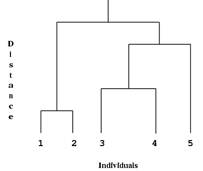
Produce Dendrogram and Clusters
Hierarchical cluster analysis can be represented by a tree that shows at which distance the clusters merge. Such a tree is known as a dendrogram; see Everitt (1974) and Krzanowski (1990). A simple example is
Figure 1
The end points of the dendrogram represent the individuals that have been clustered.
Alternatively, the information from the tree can be used to produce either a chosen number of clusters or the clusters that exist at a given distance. The latter is equivalent to taking the dendrogram and drawing a line across at a given distance to produce clusters. |
2.2.2 Non-hierarchical clustering
Non-hierarchical cluster analysis usually forms a given number of clusters from the data. There is no requirement that if first and then clusters were requested then the clusters would be formed from the clusters.
Most non-hierarchical methods of cluster analysis seek to partition the set of individuals into a number of clusters so as to optimize a criterion. The number of clusters is usually specified prior to the analysis. One commonly used criterion is the within-cluster sum of squares. Given
individuals with
variables measured on each individual,
, for
and
, the within-cluster sum of squares for
clusters is
where
is the set of objects in the
th cluster and
is the mean for the variable
over cluster
. Starting with an initial allocation of individuals to clusters, the method then seeks to minimize
by a series of re-allocations. This is often known as
-means clustering.
In the
-means case individuals belong to a single cluster and are excluded from all remaining clusters. Alternatively, probabilities of cluster membership can be estimated and each cluster can have its own distributional properties. For example, given an initial set of probabilities, the Normal (Gaussian) mixture model uses the E–M method of
Dempster et al. (1977) to maximize the sum of log-likelihoods over
clusters for a given covariance model ranging from pooled variance to individual covariance matrices.
2.2.3 Discriminant analysis
Discriminant analysis is concerned with the
allocation of objects to
groups on the basis of observations on those objects using an allocation rule. This rule is computed from observations coming from a
training set in which group membership is known. The allocation rule is based on the distance between the object and an estimate of the location of the groups. If
variables are observed and the vector of means for the
th group in the training set are
then the usual measure of the distance of an observation,
, from the
th group mean is given by Mahalanobis squared distance
where
is either the within-group variance-covariance matrix,
, for the
objects in the
th group, or a pooled variance-covariance matrix,
, computed from all
objects from all groups where
If the within-group variance-covariance matrices can be assumed to be equal then the pooled variance-covariance matrix can be used. This assumption can be tested using the test statistic
where
For large
,
is approximately distributed as a
variable with
degrees of freedom; see
Morrison (1967).
In addition to the distances, a set of prior probabilities of group membership, , for , may be used. The prior probabilities reflect your view as to the likelihood of the objects coming from the different groups.
It is generally assumed that the
variables follow a multivariate Normal distribution with, for the
th group, mean
and variance-covariance matrix
. If
is the probability of observing the observation
from group
, then the posterior probability of belonging to group
is
An observation is allocated to the group with the highest posterior probability.
In the estimative approach to discrimination, the parameters and in are replaced by their estimates calculated from the training set. If it is assumed that the within-group variance-covariance matrices are equal then the linear discriminant function is obtained; otherwise if it is assumed that the variance-covariance matrices are unequal then the quadratic discriminant function is obtained.
In the Bayesian
predictive approach, a non-informative prior distribution is used for the parameters giving the posterior distribution for the parameters from the training set,
, of,
. A predictive distribution is then obtained by integrating
over the parameter space. This predictive distribution,
, then replaces
to give
In addition to allocating the objects to groups, an atypicality index for each object and for each group can be computed. This represents the probability of obtaining an observation more typical of the group than that observed. A high value of the atypicality index for all groups indicates that the observation may in fact come from a group not represented in the training set.
Alternative approaches to discrimination are the use of canonical variates and logistic discrimination. Canonical variate analysis is described above and as it seeks to find the directions that best discriminate between groups these directions can also be used to allocate further observations. This can be viewed as an extension of Fisher's linear discriminant function. This approach does not assume that the data is Normally distributed, but Fisher's linear discriminant function may not perform well on non-Normal data. In the case of two groups, logistic regression can be performed with the response variable indicating the group allocation and the variables in the discriminant analysis being the explanatory variables. Allocation can then be made on the basis of the fitted response value. This is known as logistic discrimination and can be shown to be valid for a wide range of distributional assumptions.
2.2.4 Scaling methods
Scaling methods seek to represent the observed dissimilarities or distances between objects as distances between points in Euclidean space. For example if the distances between objects A, B and C were , and , the distances could be represented exactly by three points in two-dimensional space. Only their relative positions would be important, the whole configuration of points could be rotated or shifted without effecting the distances between the points. If a one-dimensional representation was required, the ‘best’ representation might give distances of and , which may be an adequate representation. If the distances were , and then these distances could not be exactly represented in Euclidean space, even in two dimensions, the best representation being the three points in a straight line giving distances , and .
In practice, the use of scaling methods has to decide upon the number of dimensions in which the data is to be represented. The smaller the number the easier it will be to assimilate the information. The chosen number of dimensions needs to give an adequate representation of the data but will often not give an exact representation because either the number of chosen dimensions is too small or the data cannot be represented in Euclidean space.
Two basic methods are available depending on the nature of the dissimilarities or distances being analysed. If the distances can be assumed to satisfy the metric inequality
then the distances can be represented exactly by points in Euclidean space and the technique known as metric scaling, classical scaling or principal coordinate analysis can be used. This technique involves the computing of the eigenvalues of a matrix derived from the distance matrix. The eigenvectors corresponding to the
largest positive eigenvalues gives the best
dimensions in which to represent the objects. If there are negative eigenvalues then the distance matrix cannot be represented in Euclidean space.
Instead of the above approach of requiring the distances from the points to match the distances from the objects as closely as possible, sometimes only a rank order equivalence is required. That is, the
th largest distance between objects should, as far as possible, be represented by the
th largest distance between points. This would be appropriate when the dissimilarities are based on subjective rankings. For example, if the objects were foods then a number of judges rank the foods for different qualities such as taste and texture, the resulting distances would not necessarily obey the metric inequality, but the rank order would be significant. Alternatively, by relaxing the requirement from matching distances to rank order equivalence only, the number of dimensions required to represent the distance matrix may be decreased. The requirement of rank order equivalence leads to non-metric or ordinal multidimensional scaling. The criterion used to measure the closeness of the fitted distance matrix to the observed distance matrix is known as STRESS, which is given by
where
is the Euclidean squared distance between the computed points
and
, and
is the fitted distance obtained when
is monotonically regressed on the observed distances
; that is,
is monotonic relative to
and is obtained from
with the smallest number of changes. Thus STRESS is a measure of by how much the set of points preserve the order of the distances in the original distance matrix, and non-metric multidimensional scaling seeks to find the set of points that minimize the STRESS.
3 Recommendations on Choice and Use of Available Routines
See
Section 4 for a list of routines available in this Chapter.
Note also that
G02GBF will fit a logistic regression model and can be used for logistic discrimination.
4 Functionality Index
| Canonical correlation analysis | | G03ADF |
| Canonical variate analysis | | G03ACF |
| compute distance matrix | | G03EAF |
| allocation of observations to groups, following G03DAF | | G03DCF |
| test for equality of within-group covariance matrices | | G03DAF |
| maximum likelihood estimates of parameters | | G03CAF |
| Principal component analysis | | G03AAF |
| orthogonal rotations for loading matrix | | G03BAF |
| multidimensional scaling | | G03FCF |
| principal coordinate analysis | | G03FAF |
| Standardize values of a data matrix | | G03ZAF |
5 Auxiliary Routines Associated with Library Routine Parameters
None.
6 Routines Withdrawn or Scheduled for Withdrawal
None.
7 References
Chatfield C and Collins A J (1980) Introduction to Multivariate Analysis Chapman and Hall
Dempster A P, Laird N M and Rubin D B (1977) Maximum likelihood from incomplete data via the algorithm (with discussion) J. Roy. Statist. Soc. Ser. B 39 1–38
Everitt B S (1974) Cluster Analysis Heinemann
Gnanadesikan R (1977) Methods for Statistical Data Analysis of Multivariate Observations Wiley
Hammarling S (1985) The singular value decomposition in multivariate statistics SIGNUM Newsl. 20(3) 2–25
Kendall M G and Stuart A (1976) The Advanced Theory of Statistics (Volume 3) (3rd Edition) Griffin
Krzanowski W J (1990) Principles of Multivariate Analysis Oxford University Press
Lawley D N and Maxwell A E (1971) Factor Analysis as a Statistical Method (2nd Edition) Butterworths
Morrison D F (1967) Multivariate Statistical Methods McGraw–Hill